

Volume 16, Issue 6 (November & December 2025)
BCN 2025, 16(6): 1081-1096 |
Back to browse issues page


Download citation:
BibTeX | RIS | EndNote | Medlars | ProCite | Reference Manager | RefWorks
Send citation to:


BibTeX | RIS | EndNote | Medlars | ProCite | Reference Manager | RefWorks
Send citation to:
Valizadeh S A, Cheetham M, Mohammadi A. DCM-ML: An Electroencephalography-based Classifier for Early Diagnosis of Schizophrenia Based on Dynamic Connectivity Matrices and Machine Learning Algorithms. BCN 2025; 16 (6) :1081-1096
URL: http://bcn.iums.ac.ir/article-1-3312-en.html
URL: http://bcn.iums.ac.ir/article-1-3312-en.html


1- Student Research Committee, Baqiyatallah University of Medical Sciences, Tehran, Iran.
2- Department of Internal Medicine, University Hospital Zurich, Zurich, Switzerland.
3- Neuroscience Research Center, Baqiyatallah University of Medical Sciences, Tehran, Iran.
2- Department of Internal Medicine, University Hospital Zurich, Zurich, Switzerland.
3- Neuroscience Research Center, Baqiyatallah University of Medical Sciences, Tehran, Iran.
Keywords: Event-related potentials (ERP), Diagnosis, Schizophrenia (SZ), Effective connectivity, Machine learning (ML), Classification
Full-Text [PDF 1380 kb]
| Abstract (HTML)
Full-Text:
Introduction
Schizophrenia (SZ) is a chronic mental disorder with a polygenic basis and an 80% heritability rate. It is characterized by symptoms, such as hallucinations, delusions, disorganized behavior, and progressive cognitive impairments (Mohammadi et al., 2018). It affects approximately 20 million individuals worldwide (James et al., 2018). Early diagnosis and intervention can have a profound impact on the lives of individuals affected. Early diagnosis allows for prompt intervention of psychotic symptoms (e.g. hallucinations, delusions, and disorganized thinking) before they become more severe, improves outcomes and long-term prognosis (e.g. daily life functioning, stability in social, academic, or work life), and prevents or delays relapses and lessens the likelihood of hospital admissions (Correll et al., 2018; Jääskeläinen et al., 2013; Mcgrath et al., 2008; Millier et al., 2014). Early diagnosis can also help to lessen the disabling aspects of the disorder (e.g. cognitive impairments or social isolation) and improve the quality of life (QoL) for patients and their families (Hor & Taylor, 2010).
Although the timely detection of SZ is crucial, it relies heavily on manual evaluation during clinical assessment (Nieuwenhuis et al., 2012). This conventional approach to clinical diagnosis is challenging due to the high heterogeneity of SZ (Orsolini et al., 2022). SZ can manifest differently across individual patients and throughout the disease, with some patients predominantly presenting positive and others negative and cognitive symptoms (Krauss et al., 2022). SZ can also show symptom overlap with other psychiatric disorders (e.g. depression), making differential diagnosis difficult without a comprehensive understanding of the patient’s medical history (Krauss et al., 2022). The subjective nature of manual evaluation is prone to human error and time-consuming (Devries & Delespaul, 1989).
Symptom onset in SZ typically occurs during adolescence and early adulthood (ages 14-30). The time between symptom onset and diagnosis and treatment is consistently one of the best predictors of later prognosis (McGlashan, 1999). The prodromal stage, during which initial symptoms may manifest, is a critical period for identifying and intervening in the progression of SZ. While cognitive symptoms can be apparent even before this stage, their detection for diagnostic purposes is especially challenging due to their ambiguity, as they are often mild or nonspecific.
When symptoms are ambiguous, individuals at risk of SZ may show irregularities in resting-state and task-related electroencephalography (EEG) activity (De Bock et al., 2020; Narayanan et al., 2014). These can include alterations in the temporal dynamics, coordination, and functional connectivity between different brain regions (e.g. instability in dynamic functional connectivity, hypo- and hyper-connectivity) compared to healthy individuals (Aubonnet et al., 2024; Cinelli et al., 2018; Koshiyama et al., 2020; de O. Toutain, et al., 2023; Yeh et al., 2023). Altered brain activity patterns may provide valuable insights into the likelihood of developing SZ.
We explored the feasibility of a novel approach to EEG dynamic analysis based on estimates of functional or practical brain connectivity, combined with machine learning (ML) techniques, to aid early diagnosis of SZ. The rationale for applying EEG dynamic analysis for SZ detection is that SZ may be considered as a disorder of brain network organization (Rubinov & Bullmore, 2013). In the present study, we reapplied a novel feature extraction approach, dynamic connectivity matrices (DCM), and utilized the generated features in combination with an ML algorithm previously developed to identify, based on their unique patterns of dynamic functional connectivity in EEG (Valizadeh et al., 2019). Standard EEG data were acquired from a clinically well-characterized cohort of adult patients. Using EEG and event-related potential (ERP) data, the expectation was that this approach to EEG dynamic analysis would accurately distinguish individuals with SZ from those without. To inform further development of this approach, we asked which combination of metrics is most informative for accurately classifying SZ. The evaluation criteria were the accuracy, sensitivity, and specificity of ML-based classification of clinically diagnosed patients with SZ and healthy individuals.
Materials and Methods
Dataset
We conducted a retrospective analysis of EEG data from 81 participants, sourced from a publicly accessible, Kaggle dataset. The EEG dataset used in this study was obtained from a publicly Kaggle dataset. According to the dataset description, informed consent was obtained from all participants for further use, and the data were fully anonymized. Therefore, no additional ethical approval or consent was required for its use in this study. However, all methods and analyses were conducted in accordance with the relevant guidelines and regulations, and the study protocol was approved by the Research Ethics Committee of Baqiyatallah University of Medical Sciences. This dataset includes EEG signals acquired from 49 SZ patients (41 males, between 22 and 63 years, Mean±SD 40±13.5) (17 in early stages and 32 in chronic stages of the disorder) and 32 healthy controls (26 males, between 22 and 63 years, Mean±SD 38.2±13). Data were acquired while participants performed a passive (auditory-only) condition of a basic auditory listening task. All patients were clinically diagnosed using the structured clinical interview for the diagnostic and statistical manual of mental disorders, fourth edition (DSM-IV) (SCID). Patients and healthy controls had no other diagnoses.
Data acquisition
EEG data were captured with a 64-channel ActiveTwo Biosemi system (Metting van Rijn et al., 1990) and cap, using the 10-10 international system, while participants engaged in the auditory listening task. This task entailed the presentation of 100 auditory stimuli (1000 Hz tones at 80 dB SPL for 50 ms.) with inter-stimulus intervals varying between 1000 and 2000 ms. EEG signals were recorded continuously and divided into separate ERP epochs of 3000 ms. Those were synchronized with the onset of each tone. The dataset also includes data acquired from an auditory-motor task (Ford et al., 2014; Pinheiro et al., 2020), which was not used in the present study. The data were collected at a sampling frequency of 1024 Hz and down-sampled to 512 Hz.
EEG preprocessing and epoching
The EEG dataset was originally preprocessed and cleaned for a previously published study (Barros et al., 2022; Ford et al., 2014) and further processed and cleaned by the same authors prior to public release. Utilizing a publicly available dataset promotes research transparency, facilitates reproducibility, and supports further investigation by other researchers.
The preprocessing steps included re-referencing to averaged earlobe electrodes, band-pass filtering between 0.5 and 15 Hz, and independent component analysis to identify and remove ocular and muscular artifacts. A regression-based algorithm was applied to correct for eye movement and blink activity across all scalp channels. Artifact rejection was performed using a ±100 µV threshold at each electrode, and non-physiological channels were interpolated based on established spatial criteria. These procedures ensured high-quality, artifact-free EEG data suitable for connectivity analysis.
For this study, the preprocessed EEG signals were segmented into 3000-ms epochs, each time-locked to the onset of the auditory stimulus. Baseline correction was applied using the window beginning 600 ms to 500 ms before tone onset.
Signal processing and epochs
Unlike traditional ERP analysis, which relies on averaging epochs to extract features, our approach treated each epoch as an independent sample. This single-trial analysis significantly expanded the dataset size, enabling the model to capture subtle inter-trial variability in neural activity. This is advantageous for studying complex neurological disorders, such as SZ, where subtle differences in neural responses may be obscured by averaging. By analyzing each epoch individually, finer-grained neural patterns were sought in line with recent advancements that emphasize the importance of trial-to-trial variability for capturing brain function (Huang et al., 2018; Ho, 1998; Valizadeh et al., 2018).
The epochs were 3000 ms in length and time-locked to the onset of the auditory stimulus (i.e. the tone). Granger causality was computed for the 3000-ms epoch, yielding 64×64 matrices for each epoch. The workflow illustrates the processing of EEG, including cleaning and epoching into stable segments representing event-related potentials (ERPs) for both training and testing. Coherence Granger causality was applied to each epoch to assess directional information flow between 64 EEG electrodes in the time domain, producing a 64×64 coherence matrix indicative of pairwise electrode connectivity. These matrices served as features for a random forest (RF) classifier. Classification assessment involved a voting process across participants, trained on the training participants, and evaluated on each event in the test participant separately.
Feature extractor
Our classification framework is based on a novel and previously validated subject identification method (Valizadeh et al., 2019). This method uses surface-level (electrode-based) functional connectivity in the time domain, computed over short, overlapping temporal windows, and generates temporal DCMs that capture the evolving patterns of interaction among EEG electrodes. Within each temporal window, the statistical relationship, whether correlational or causal, is quantified between pairs of EEG time series. This dynamic representation enables fine-grained tracking of brain network changes over time and has been adopted in the present study as input features for classifying SZ-related neural activity.
The clean EEG data were divided into epochs, each deemed sufficiently stable for connectivity analysis. Within each epoch, coherence Granger causality was used to assess interactions between EEG signals from different electrodes in the time domain (Figure 1). Causation, or directional connectivity, was used to evaluate the extent to which the activity in one EEG electrode could predict the activity in another. All analyses were performed in the time domain, except for the initial filtering stage. An iterative method was employed to determine the interaction between each seed electrode and every other electrode, producing a 64×64 matrix that illustrates the pairwise connectivity among all electrode pairs.

Granger causality is a statistical method used to assess whether one time series can predict another. If past values of variable X significantly improve the prediction of variable Y— beyond what is possible using Y’s own history—X is said to “Granger-cause” Y. This is typically evaluated using a linear regression model, where the target time series is regressed on its own past values and those of another series; statistical significance of the latter indicates predictive influence.
In EEG analysis, Granger causality is applied to identify directional interactions between brain regions, providing insight into neural connectivity associated with cognitive processes and disorders such as SZ (Gao et al., 2020; Huang et al., 2018). Importantly, Granger causality reflects predictive, not necessarily direct, causal relationships, suggesting information flow from one electrode to another.
Granger Causality is computed as follows:
Model specification:
Two time series, X and Y, are examined.
A regression model is constructed for Y based on its previous values in conjunction with the past values of Y.
Lag selection: Identify the appropriate lags for the time series. This can be achieved using metrics, such as the Akaike information criterion (AIC) or the Bayesian information criterion (BIC).
Regression analysis: Conduct two regression analyses:
Model 1:
𝑌𝑡=𝑎0+𝑎1𝑌𝑡−1+𝑎2𝑌𝑡−2+....+𝑎𝑛𝑌𝑡−𝑛
Model 2: Model 2 includes past values of X.

Hypothesis testing: The null hypothesis 𝐻0 posits that X does not Granger-cause Y (i.e. the coefficients 𝑐1, 2, ... are equal to zero).
Implement an F-test to compare the two models. If the inclusion of X substantively enhances the predictive capacity for Y, the null hypothesis is rejected, indicating that X Granger-causes Y.
To ensure consistency and avoid model complexity or overfitting, we did not perform individual model selection using information criteria, such as the Bayesian Information Criterion (BIC) or the Akaike Information Criterion (AIC). Instead, we set the model lag order to a fixed value of 10 across all participants and conditions. This approach simplifies the analysis pipeline and ensures cross-subject comparability while remaining within a range adequate to capture relevant temporal dependencies in EEG time series data.
ML procedures
The number of participants in each group is unbalanced, with 32 healthy individuals and 49 individuals with SZ. To prevent unbalanced learning, we used the healthy control (HC) sample, selected half for training, and matched the SZ group with an equal number of participants. This led to 16 participants from each group being randomly selected for training. We subsequently categorized the remaining healthy participants and individuals with SZ. This approach reduces the classifier’s performance but improves its reliability when evaluating each additional participant. The classifiers are fed directly by the connectivity matrices. Every training step, along with the classifiers, was performed on the training set. The number of epochs for each participant remains the same.
To mitigate the potential for overfitting, a particular concern in smaller datasets with k-fold cross-validation, we employed a 50/50 train-test split. This approach aimed to maximize data utilization while minimizing the risk of overfitting. Prior to classification, a feature selection phase was conducted to refine the feature space and potentially enhance model performance. Independent two-sample t-tests were performed on the training datasets to identify connectivity features exhibiting statistically significant differences (P<0.05) between the defined groups: HC and individuals with SZ. Only these features were retained AS input features for the classification algorithms.
This feature selection approach was designed to reduce dimensionality, minimize noise, and improve model performance by focusing on the most salient and discriminatory features. This enhances the model’s ability to accurately categorize individuals into their respective diagnostic groups and its interpretability by highlighting neural connectivity patterns associated with SZ.
The feature set comprised 64×64×100 epochs, indicating that each participant contributed 100 samples, each with 64×64 features. Consequently, the training set for each class consisted of 16×100 samples, each with 1 * 4096 elements (i.e. a 1×4096 feature vector). The final training set was structured as a matrix with 3200 rows (samples) and 4096 columns (connections). An additional column was appended to the data as the class label, indicating group membership (SZ or non-SZ). A t-test was conducted based on this class label. The classification of each epoch within the test set was performed independently. A participant was classified as SZ if a majority of epochs (at least 51 out of 100) were labeled as SZ; otherwise, they were classified as non-SZ.
Classification
The classification process was performed on all test epochs. The classification set was determined according to the following criteria: Participants were labeled SZ or non-SZ based on the majority classification of their epochs. Those with an equal number of SZ and non-SZ epochs would have been designated as unknown; however, no participants fell into this category in the current dataset.
Classifier
The RF algorithm (Ho, 1998) is a robust ML algorithm and particularly effective for classification tasks, including medical diagnosis prediction. It operates by constructing an ensemble of decision trees, each trained on a random subset of the data. This bootstrapping approach ensures that each tree learns diverse aspects of the data, mitigating overfitting and improving generalization. In predicting, every tree in the forest votes, and the most common class or the average prediction is selected as the result. This collective characteristic provides multiple benefits (Valizadeh et al., 2019):
Great precision: The combined knowledge of several trees frequently results in exact predictions.
Resilience to noise: The algorithm remains strong against noisy data and outliers because of the ensemble’s averaging impact.
Evaluation of feature importance: RF offers insights into the significance of various features, assisting in feature selection and aiding in comprehending the fundamental patterns present in the data.
Managing absent data: It efficiently manages absent data in the dataset.
Scalability: RF effectively manages extensive datasets, rendering it appropriate for practical applications.
Classification assessment
Accuracy assesses the overall correctness of a model’s predictions, i.e. the ratio of correctly classified cases to the total number of instances. Although high accuracy often suggests strong performance, it can be deceptive in imbalanced datasets where one class greatly exceeds the other. Sensitivity, also known as recall, measures the model’s ability to accurately identify positive cases, which is essential when the penalty for failing to detect a positive instance is significant. On the other hand, specificity measures the model’s ability to accurately identify negative instances, which is essential when misclassifying a negative instance can lead to serious outcomes. The F1-score, the harmonic mean of precision and recall, provides a single metric that balances both factors, especially useful for imbalanced datasets.
Selecting the appropriate metric is related to accurately detecting both positive and negative cases. Note that there is frequently a compromise between sensitivity and specificity; enhancing one usually results in a decline of the other. In addition, accuracy may be misleading in imbalanced datasets, as metrics such as sensitivity, specificity, and F1-score provide a more nuanced assessment of model effectiveness.
An additional strategy was implemented to evaluate the robustness of the classification outcomes. This strategy is based on the following considerations. If a neural network is trained to recognize stimuli, its performance should remain consistent when identifying stimuli, such as faces, from various angles, under different lighting conditions, or when presented with partial facial features (Valizadeh et al., 2018, Valizadeh et al., 2019). This means that the classifier must retain accuracy even when target stimuli are altered or degraded. To replicate these scenarios, white Gaussian noise was incrementally added to the test dataset’s connectivity matrices. Initially, the classification analysis was conducted without noise (0% noise level). Subsequently, noise was linearly added to all features in increments of 5% and progressing to 45%. This process resulted in nine distinct ten conditions (0%, 5%, 10%, 15%, …, 45%), each subjected to separate classification evaluations.
Results
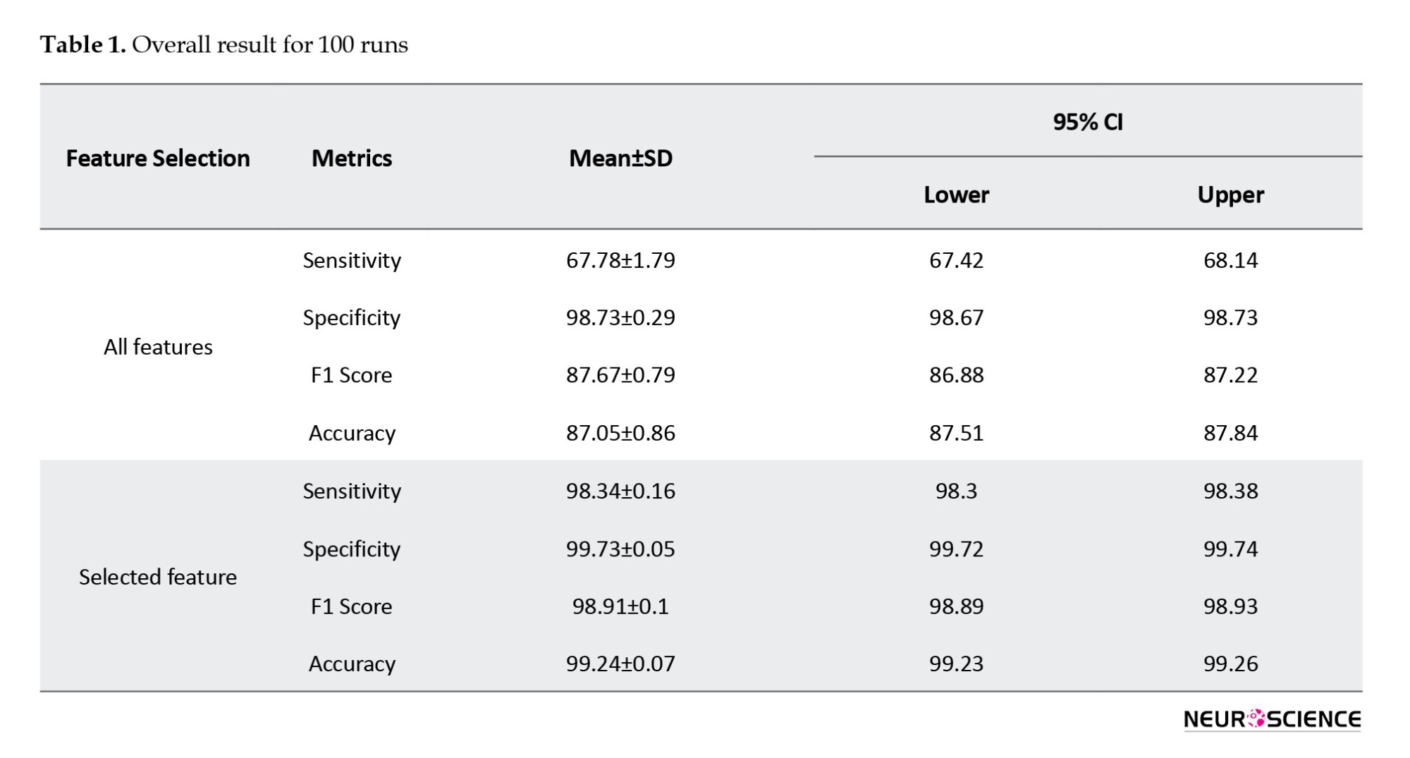
The RF model showed very high overall performance through various assessment metrics, evaluated over 100 iterations to reduce the impact of overfitting and random effects (Table 1). Sensitivity, a metric reflecting the model’s ability to correctly identify positive instances, reached 0.98, with a 95% confidence interval (CI) of 98.34±0.04%. This indicates that the model was highly accurate in detecting the target condition when present. Similarly, specificity, which evaluates the model’s ability to correctly identify negative instances, achieved a perfect score of 1.00 with 99.73±0.01% CI, demonstrating that the model did not mislabel any negative cases. The F1 score, balancing precision and recall, was also high at 0.99 with 98.91±0.02% CI, emphasizing the model’s strong predictive capacity. Finally, the overall accuracy of the model, determined as the proportion of accurate predictions, was 0.99 (99.24±0.02%), indicating that the model generated highly accurate predictions on the dataset.
Test train rate
Figure 2 shows the impact of the test rate on classification performance. Notably, the RF classifier shows very high performance even with relatively limited training sample sizes. This is consistent with previous studies that highlighted the effectiveness of RF classifiers in handling imbalanced datasets and in generalizing well to unseen data (Fawagreh et al., 2014).
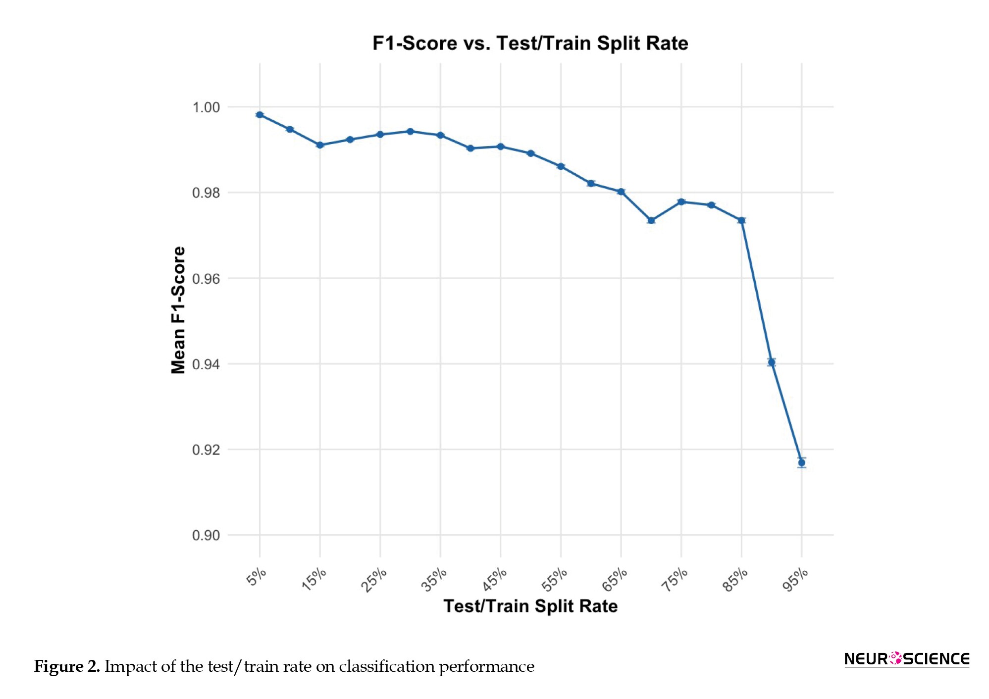
However, when the testing rate approaches very high levels (0.09 and 0.95), classification accuracy declines. This trend shows that while RF classifiers are robust against data distribution, significant imbalances can still negatively influence their performance. This finding aligns with current research, suggesting that imbalanced datasets pose challenges for ML models, potentially leading to biased results. To confirm that the observed performance trends were not due to random factors, we systematically adjusted the test rate from 5% to 95% of the overall epochs (Table 2). This method enabled us to evaluate the classifier’s strength across various data distributions. Despite a test rate of 95%, the RF classifier obtained an F1-score of 92%, indicating its ability to handle imbalanced datasets.

Noise stability
Figure 3 shows how rising levels of white Gaussian noise affect the classification performance of two sets of features: “All features” and “selected features noise was progressively introduced to the connectivity matrices of the test dataset, simulating scenarios in which target stimuli are modified or compromised. The x-axis shows the percentage of introduced noise, ranging from 0% (no noise) to 45%, while the y-axis displays the F1-score, a metric of classification accuracy. As the noise percentage increases, both feature sets exhibit a decline in F1-score, indicating reduced classification effectiveness. However, the “selected features” (blue line) demonstrate greater resilience to noise, consistently achieving higher F1 Scores than the “all features” set (red line) across all noise levels. This suggests that the “selected features” are more robust against the detrimental effects of noise and provide more reliable classification, even when the data is compromised.
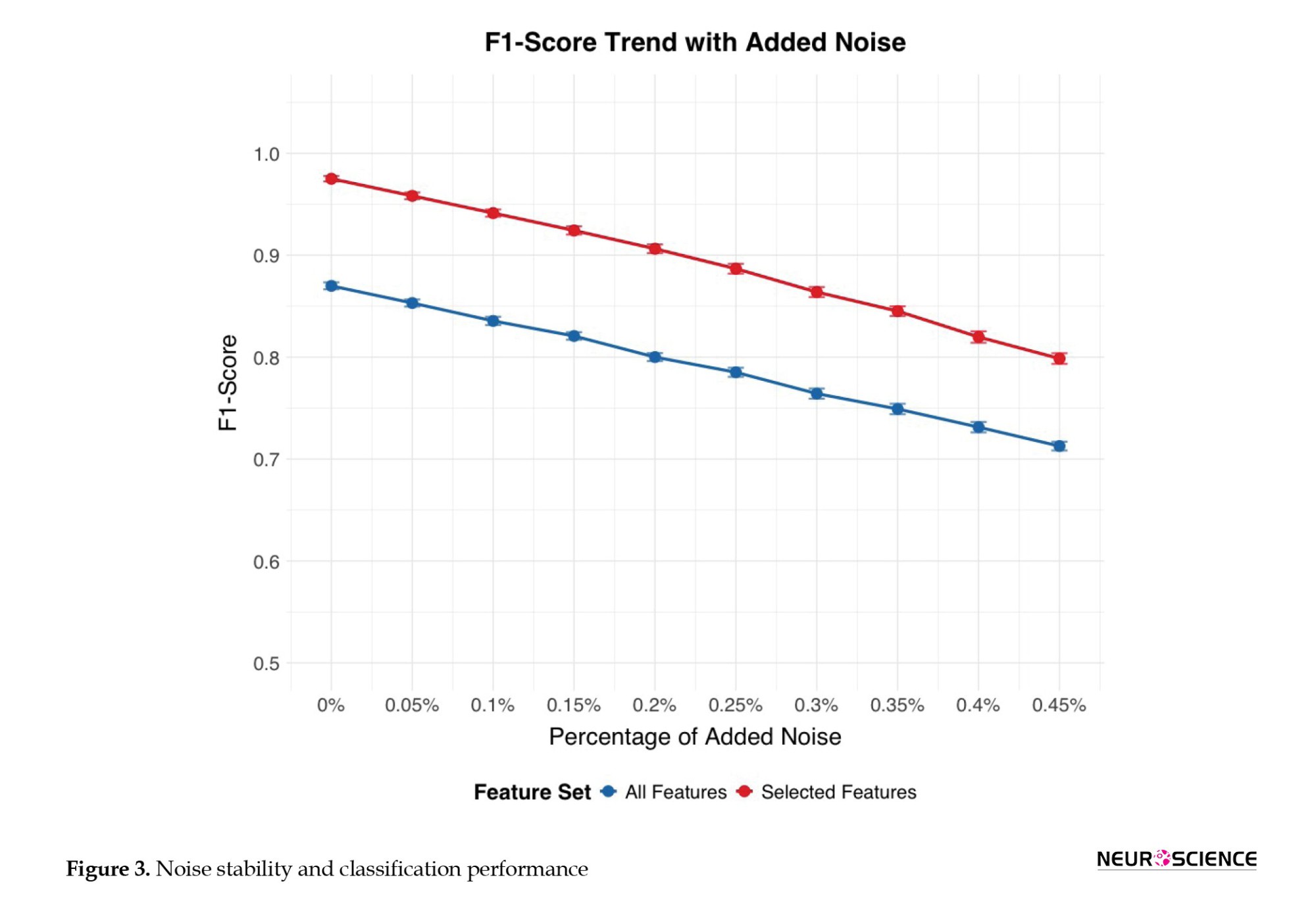
This figure shows, for all (blue line) and selected features (red line), the percentage of added noise, (ranging from 0% [no noise] to 45%) on the x-axis, against the F1-score (i.e. classification accuracy) on the y-axis. Error bars represent CIs of the F1-score calculated over 100 runs or folds.
Electrode contribution to classification
Through a comprehensive analysis of Granger causality across all 64×64 electrode pair combinations, we identified 2,777 connections that exhibited statistically significant differences between the HC and SZ groups (P values ranging from 0.049 to 10-74) based on trained datasets. Table 3 presents the most discriminatory Granger causality combinations, characterized by particularly robust statistical significance (P<10-30). To further investigate the regional brain areas most implicated in these group differences, we created a frequency table. This table is based on all Granger causality combinations that demonstrate significant group separation (P<0.05). It counts how often each electrode appears as either a predictor or a predicted region across these significant connections. The most frequently identified electrodes from this process are presented in a subsequent table to highlight key regions involved in connectivity alterations in SZ.

Following the identification of the 2,777 statistically significant Granger causality combinations that differentiated the HC and SZ groups (P<0.05), a frequency analysis was performed to determine the most relevant electrode regions (Table 4). This table reports the top ten electrodes ranked by their total frequency of appearance in significant connections. For each electrode (column 1), the table shows its frequency as a predictor electrode (column 2), its frequency as a predicted electrode (column 3), and the summed total frequency (column 4). A higher total frequency indicates greater involvement in group-discriminating Granger-causality relationships.

Discussion
The present study was guided by two primary research questions: Is it possible to identify SZ using our novel EEG-based ML classifier based on DCM, and which combination of metrics is most informative for classifying SZ? The DCM-ML approach identified SZ with a very high degree of accuracy, approaching 100%. Our findings indicate that only a subset of metrics is required to achieve effective classification of individual participants, highlighting the efficiency and specificity of the selected features. These results underscore the potential of using targeted metrics to enhance the precision of SZ detection.
The RF model demonstrated very high performance across various metrics. It achieved a sensitivity of 0.98 (98.34±0.04%), indicating its proficiency in accurately identifying positive cases. In addition, it exhibited a perfect specificity of 1.00 (99.73±0.01%), demonstrating its ability to correctly classify negative instances without mislabeling. The model also achieved a high F1 score of 0.99 (98.91±0.02%), indicating a strong balance between precision and recall. Furthermore, the overall accuracy was 0.99 (99.24±0.02%), which is consistent with the model’s ability to generate highly accurate predictions on the dataset. These results underscore the potential of targeted metrics to enhance the precision of SZ diagnosis.
This study also assessed the stability of the proposed classification method under different conditions. The introduction of white Gaussian noise led to a gradual, but predictable, decline in classification performance. At noise levels up to 10% of the data, the accuracy remained above 95%, demonstrating considerable resilience. However, beyond 10%, the accuracy decreased more rapidly, highlighting the sensitivity of ERP-based connectivity measures to excessive noise. This underscores the importance of stringent data-acquisition protocols and noise-reduction techniques in ERP studies.
The RF classifier exhibited strong performance across different training sample sizes, demonstrating its ability to generalize effectively even with limited data. This finding is consistent with prior research, which has emphasized the robustness of RF classifiers in handling imbalanced datasets and their capacity to maintain high accuracy under constrained conditions. However, when the testing rate approached extreme values (0.09 and 0.95), classification accuracy declined. This suggests that while RF classifiers are generally resilient to variations in data distribution, significant imbalances can still adversely affect their performance (Luan et al., 2020; Valizadeh et al., 2018, 2019; Wang et al., 2016; Zhang et al., 2009).
Our findings on specific ERP components and inter-electrode connectivity patterns offer valuable insights into the neurophysiological underpinnings of SZ. Notably, our analysis revealed that a subset of electrodes (Cz, FCz, Iz, PO3, CP4, AF3, C1, O1, and POz) was particularly influential in distinguishing individuals with SZ from HC. This emphasis on a targeted set of electrodes strikes a balance between diagnostic accuracy and the practical considerations of clinical EEG procedures.
The prominence of central midline electrodes, particularly Cz and FCz, in our findings aligns with the existing literature, which emphasizes the role of these regions in SZ pathophysiology. As highlighted in the literature, Cz is consistently identified as a core component in optimal electrode subsets for SZ detection, likely due to its sensitivity to global neural dynamics and altered connectivity patterns in resting-state paradigms (Becske et al., 2024; Mahato et al., 2021). The involvement of FCz, while sometimes represented by the functionally proximal Fz in standard montages, further supports the importance of frontocentral activity in capturing auditory-evoked anomalies and deficits related to auditory steady-state responses in SZ (Hirano et al., 2020). These findings suggest that disruptions in information processing and sensory integration, often observed in SZ, are reflected in the altered activity and connectivity of these central and frontocentral regions.
The present study also identified other key electrodes, including those in occipital (O1, POz), parietal (CP4), and frontal (AF3) regions, as contributing to accurate classification. The involvement of O1 aligns with evidence of visual processing abnormalities and disruptions of the default mode network in SZ (Becske et al., 2024; Zeltser et al., 2024). While POz, CP4, and AF3 may not have been as extensively studied in classification frameworks, their inclusion in our model and their presence in network analyses suggest their potential role in capturing specific aspects of the disorder, such as visuospatial integration deficits (POz), right-lateralized connectivity abnormalities (CP4), and prefrontal cortex dysfunction (AF3). The inclusion of C1, near the primary somatosensory cortex, points towards possible sensorimotor integration abnormalities in SZ, though further research is needed to validate its specific contribution to classification models. The relative lack of direct evidence for Iz in the literature suggests that it has limited diagnostic value within current paradigms (Srinivasan et al., 2024). Taken together, these results indicate that a distributed network of brain regions, extending beyond the frontal cortex, contributes to the neurophysiological signature of SZ.
Imbalanced datasets pose challenges in ML. The present results align with existing literature in this regard (Paraschiv et al., 2024). The observed decline in accuracy at very high testing rates highlights the potential for biased outcomes when data distributions are significantly skewed. This emphasizes the need to carefully consider dataset composition and to apply strategies to mitigate imbalance, such as resampling techniques or algorithmic adjustments, to ensure the reliability and generalizability of classification models.
Comparison of the model with other models
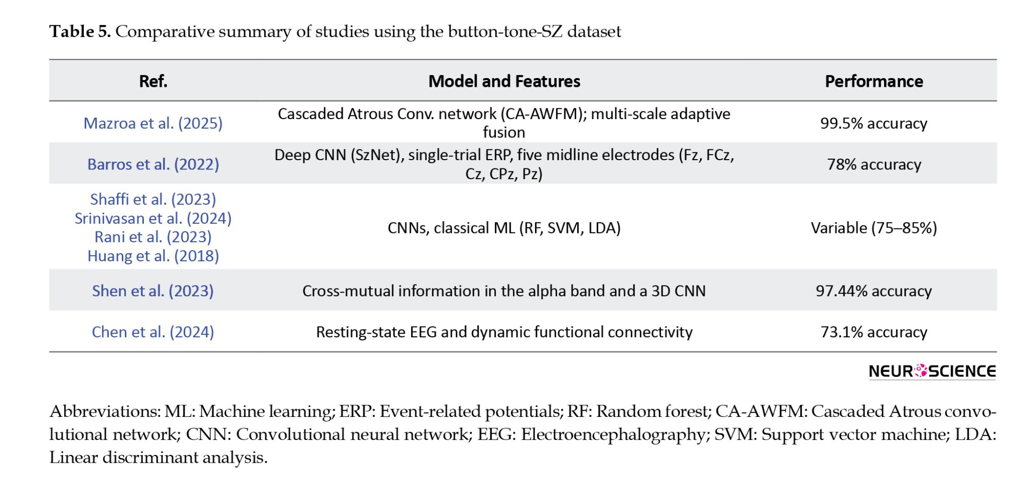
The dataset used in this study has been previously analyzed, using both traditional ML algorithms (Rani et al., 2023; Shaffi et al., 2023; Srinivasan et al., 2024) and recent deep learning methods (Paraschiv et al., 2024; Rao et al., 2025; Sahu et al., 2023; Stunnenberg et al., 2024; Swastika, 2022). These studies established performance benchmarks and demonstrated the dataset’s value for detecting neuropsychiatric disorders, such as SZ.
Although deep learning techniques have achieved high accuracy (up to 97%), their complexity, large model sizes, and high computational demands often limit their applicability in time-sensitive, real-world clinical settings.
To address this limitation, this present study presents a novel, computationally efficient ML model applied to the same dataset. This approach achieves extremely high classification accuracy (99.24%, 98.34%, and 99.73%) without requiring deep hierarchical networks or dense feature engineering. By extracting ERPs from a cognitive auditory task, we observe task-related brain dynamics and construct directional DCMs based on Granger causality. This approach also accurately maps inter-electrode information flow while preserving single-trial variability —an essential dimension usually lost to average-based or resting-state methods.
Compared to existing methods, our approach has several advantages. For instance, Chen et al. (2024) used resting-state EEG and dynamic functional connectivity to achieve multi-class classification of various psychiatric disorders with moderate accuracy (73.1%). However, their method is based on averaged DFC states and does not account for signal variability or noise resistance. In contrast, our method relies on single-trial ERP data, retaining inter-epoch variability and exhibiting significant robustness to noise with an F1-score of 92% even in the presence of 45% Gaussian noise—a point entirely unexplored in their work.
Similarly, Shen et al. (2023) employ cross-mutual information in the alpha band and a 3D CNN to discriminate SZ from resting-state EEG with 97.74% accuracy. Their approach is practical but relies on undirected, frequency-specific connectivity rather than the temporal specificity our ERP-based paradigm enables. Our model not only improves accuracy but also offers greater interpretability and clinical utility by selecting directionality patterns of connectivity and electrode-level biomarkers, particularly in fronto-central and occipito-parietal regions that are critical to SZ pathology.
A recent study (Ciprian et al., 2021) utilizing symbolic transfer entropy on resting-state EEG also achieved high performance (96.92%) with minimal features. In the absence of task engagement, however, their approach may fail to capture critical neurocognitive signatures of SZ. Our DCM-based model, with direction-aware task-evoked P300 responses, can extract functional impairments in challenging cognitive conditions and is facilitated by direction-aware DCMs, offering a more comprehensive description of inter-regional interactions. Again, our model’s noise resistance and ability to maintain subtle pathological signals through single-trial analysis position it as a more clinically viable instrument.
Compared to a range of recent studies that have employed both deep learning and classical ML techniques for SZ detection using EEG or ERP data, the present study offers a unique combination of interpretability, robustness, and clinical relevance. While several approaches report high classification accuracies, for example, 99.5% using a cascaded Atrous convolutional network (CA-AWFM) (Mazroa et al., 2025) with multi-scale feature fusion and 99.9% via ERP feature integration and demographics, these methods often rely on black-box architectures or require multimodal data inputs, which can limit clinical transparency and scalability. In contrast, our study achieves comparably high accuracy (99.24%) using a single-modality ERP dataset and a RF classifier trained on features derived from directional DCMs computed with Granger causality. This approach emphasizes inter-regional information flow, a critical neural marker often overlooked in frequency-domain or undirected methods.
While methods, such as SchizoGoogLeNet and multiple kernel learning, also achieve strong results (Castro et al., 2014; Siuly et al., 2022), they typically depend on either large-scale automated feature extraction or fusion of multiple ERP components (e.g. P300, MMN), requiring extensive preprocessing pipelines. In contrast, our model is noise-resilient, maintaining a 92% F1-score even with 45% added Gaussian noise, and uses single-trial data to preserve the subtle inter-epoch variability vital for identifying SZ-related deficits. In addition, our identification of clinically relevant electrode-level patterns in fronto-central and occipito-parietal regions makes the findings more explainable and suitable for integration into real-time or portable diagnostic tools.
While deep learning models, such as those of Mazroa et al. (2025), demonstrate impressive levels of accuracy, their complexity, limited interpretability, and reliance on resting-state signals or black-box convolutional layers hinder real-world deployment. In contrast, our method balances accuracy, interpretability, and practicality, making it well-suited for scalable clinical translation, especially for early SZ detection n settings with limited computational resources and variable signal quality.
In summary, the present approach overcomes the limitations of existing methods by combining interpretable directionality features with a high-performance yet lightweight classifier into a practical, scalable, and highly accurate method for early SZ diagnosis.
This approach has the potential to bridge algorithmic performance with real-world clinical usability.
Limitations and future work
From a clinical perspective, this approach shows promise as a complementary tool for early diagnosis of SZ. At this stage, our study serves as a proof-of-concept of our ML approach and the results should be interpreted in terms of the feasibility of this ML-based classifier for clinical application. The findings suggest that the ML-based classifier may detect early-phase EEG abnormalities associated with SZ. However, predictive models must also account for the variability in individual disease progression. Additionally, the current dataset does not allow for an assessment of whether these abnormalities overlap with other mental health conditions. Future development of the current approach should consider disease progression and comorbidities within a demographically and clinically broader and more diverse dataset than that used in this study to verify the method’s reliability and clinical applicability. This could be supported by acquiring longitudinal data to identify consistent patterns of EEG abnormalities (and changes in these patterns) prior to the prodromal phase, throughout the prodromal transition, and after the onset of psychosis. These data can serve as a foundation for developing reliable predictive markers. Although the model’s high accuracy is promising, understanding the specific features or patterns that influence its predictions is crucial. Integrating this approach with multimodal data (e.g. biomarkers and clinical evaluations) may enhance diagnostic accuracy. Further efforts to improve the model’s interpretability will be essential for its integration into clinical practice.
Conclusion
The tested approach, using a novel EEG-based classifier based on DCM and ML algorithms, marks a considerable improvement in the use of dynamic EEG analysis for SZ detection. The very high F1-score demonstrates the capability of computational methods to support psychiatric diagnostics, providing an objective and non-invasive instrument for early detection and intervention. This approach requires additional refinement and validation based on broader demographic and clinical datasets to verify its reliability and applicability.
Ethical Considerations
Compliance with ethical guidelines
All methods and analyses were conducted in accordance with the relevant guidelines and regulations, and the study protocol was approved by the Research Ethics Committee of Baqiyatallah University of Medical Sciences, Tehran, Iran (Code: IR.BMSU.BAQ.REC.1403.147).
Funding
This research did not receive any specific grants from funding agencies in the public, commercial, or not-for-profit sectors.
Authors' contributions
Study design: Marcus Cheetham and Alireza Mohammadi; Data interpretation: All authors; Writing the Python code and analyses: Seyed Abolfazl Valizadeh; Project administration, supervision, review, editing, and final approval: Alireza Mohammadi.
Conflict of interest
The authors declared no conflict of interest.
Acknowledgments
The authors express their deep gratitude to the Neuroscience Research Center at Baqiyatallah University of Medical Sciences for their valuable support and resources, with contributed significantly to the success of this study. The authors are extremely grateful to the Kaggle website for providing access to the data for the scientific community.
References
Schizophrenia (SZ) is a chronic mental disorder with a polygenic basis and an 80% heritability rate. It is characterized by symptoms, such as hallucinations, delusions, disorganized behavior, and progressive cognitive impairments (Mohammadi et al., 2018). It affects approximately 20 million individuals worldwide (James et al., 2018). Early diagnosis and intervention can have a profound impact on the lives of individuals affected. Early diagnosis allows for prompt intervention of psychotic symptoms (e.g. hallucinations, delusions, and disorganized thinking) before they become more severe, improves outcomes and long-term prognosis (e.g. daily life functioning, stability in social, academic, or work life), and prevents or delays relapses and lessens the likelihood of hospital admissions (Correll et al., 2018; Jääskeläinen et al., 2013; Mcgrath et al., 2008; Millier et al., 2014). Early diagnosis can also help to lessen the disabling aspects of the disorder (e.g. cognitive impairments or social isolation) and improve the quality of life (QoL) for patients and their families (Hor & Taylor, 2010).
Although the timely detection of SZ is crucial, it relies heavily on manual evaluation during clinical assessment (Nieuwenhuis et al., 2012). This conventional approach to clinical diagnosis is challenging due to the high heterogeneity of SZ (Orsolini et al., 2022). SZ can manifest differently across individual patients and throughout the disease, with some patients predominantly presenting positive and others negative and cognitive symptoms (Krauss et al., 2022). SZ can also show symptom overlap with other psychiatric disorders (e.g. depression), making differential diagnosis difficult without a comprehensive understanding of the patient’s medical history (Krauss et al., 2022). The subjective nature of manual evaluation is prone to human error and time-consuming (Devries & Delespaul, 1989).
Symptom onset in SZ typically occurs during adolescence and early adulthood (ages 14-30). The time between symptom onset and diagnosis and treatment is consistently one of the best predictors of later prognosis (McGlashan, 1999). The prodromal stage, during which initial symptoms may manifest, is a critical period for identifying and intervening in the progression of SZ. While cognitive symptoms can be apparent even before this stage, their detection for diagnostic purposes is especially challenging due to their ambiguity, as they are often mild or nonspecific.
When symptoms are ambiguous, individuals at risk of SZ may show irregularities in resting-state and task-related electroencephalography (EEG) activity (De Bock et al., 2020; Narayanan et al., 2014). These can include alterations in the temporal dynamics, coordination, and functional connectivity between different brain regions (e.g. instability in dynamic functional connectivity, hypo- and hyper-connectivity) compared to healthy individuals (Aubonnet et al., 2024; Cinelli et al., 2018; Koshiyama et al., 2020; de O. Toutain, et al., 2023; Yeh et al., 2023). Altered brain activity patterns may provide valuable insights into the likelihood of developing SZ.
We explored the feasibility of a novel approach to EEG dynamic analysis based on estimates of functional or practical brain connectivity, combined with machine learning (ML) techniques, to aid early diagnosis of SZ. The rationale for applying EEG dynamic analysis for SZ detection is that SZ may be considered as a disorder of brain network organization (Rubinov & Bullmore, 2013). In the present study, we reapplied a novel feature extraction approach, dynamic connectivity matrices (DCM), and utilized the generated features in combination with an ML algorithm previously developed to identify, based on their unique patterns of dynamic functional connectivity in EEG (Valizadeh et al., 2019). Standard EEG data were acquired from a clinically well-characterized cohort of adult patients. Using EEG and event-related potential (ERP) data, the expectation was that this approach to EEG dynamic analysis would accurately distinguish individuals with SZ from those without. To inform further development of this approach, we asked which combination of metrics is most informative for accurately classifying SZ. The evaluation criteria were the accuracy, sensitivity, and specificity of ML-based classification of clinically diagnosed patients with SZ and healthy individuals.
Materials and Methods
Dataset
We conducted a retrospective analysis of EEG data from 81 participants, sourced from a publicly accessible, Kaggle dataset. The EEG dataset used in this study was obtained from a publicly Kaggle dataset. According to the dataset description, informed consent was obtained from all participants for further use, and the data were fully anonymized. Therefore, no additional ethical approval or consent was required for its use in this study. However, all methods and analyses were conducted in accordance with the relevant guidelines and regulations, and the study protocol was approved by the Research Ethics Committee of Baqiyatallah University of Medical Sciences. This dataset includes EEG signals acquired from 49 SZ patients (41 males, between 22 and 63 years, Mean±SD 40±13.5) (17 in early stages and 32 in chronic stages of the disorder) and 32 healthy controls (26 males, between 22 and 63 years, Mean±SD 38.2±13). Data were acquired while participants performed a passive (auditory-only) condition of a basic auditory listening task. All patients were clinically diagnosed using the structured clinical interview for the diagnostic and statistical manual of mental disorders, fourth edition (DSM-IV) (SCID). Patients and healthy controls had no other diagnoses.
Data acquisition
EEG data were captured with a 64-channel ActiveTwo Biosemi system (Metting van Rijn et al., 1990) and cap, using the 10-10 international system, while participants engaged in the auditory listening task. This task entailed the presentation of 100 auditory stimuli (1000 Hz tones at 80 dB SPL for 50 ms.) with inter-stimulus intervals varying between 1000 and 2000 ms. EEG signals were recorded continuously and divided into separate ERP epochs of 3000 ms. Those were synchronized with the onset of each tone. The dataset also includes data acquired from an auditory-motor task (Ford et al., 2014; Pinheiro et al., 2020), which was not used in the present study. The data were collected at a sampling frequency of 1024 Hz and down-sampled to 512 Hz.
EEG preprocessing and epoching
The EEG dataset was originally preprocessed and cleaned for a previously published study (Barros et al., 2022; Ford et al., 2014) and further processed and cleaned by the same authors prior to public release. Utilizing a publicly available dataset promotes research transparency, facilitates reproducibility, and supports further investigation by other researchers.
The preprocessing steps included re-referencing to averaged earlobe electrodes, band-pass filtering between 0.5 and 15 Hz, and independent component analysis to identify and remove ocular and muscular artifacts. A regression-based algorithm was applied to correct for eye movement and blink activity across all scalp channels. Artifact rejection was performed using a ±100 µV threshold at each electrode, and non-physiological channels were interpolated based on established spatial criteria. These procedures ensured high-quality, artifact-free EEG data suitable for connectivity analysis.
For this study, the preprocessed EEG signals were segmented into 3000-ms epochs, each time-locked to the onset of the auditory stimulus. Baseline correction was applied using the window beginning 600 ms to 500 ms before tone onset.
Signal processing and epochs
Unlike traditional ERP analysis, which relies on averaging epochs to extract features, our approach treated each epoch as an independent sample. This single-trial analysis significantly expanded the dataset size, enabling the model to capture subtle inter-trial variability in neural activity. This is advantageous for studying complex neurological disorders, such as SZ, where subtle differences in neural responses may be obscured by averaging. By analyzing each epoch individually, finer-grained neural patterns were sought in line with recent advancements that emphasize the importance of trial-to-trial variability for capturing brain function (Huang et al., 2018; Ho, 1998; Valizadeh et al., 2018).
The epochs were 3000 ms in length and time-locked to the onset of the auditory stimulus (i.e. the tone). Granger causality was computed for the 3000-ms epoch, yielding 64×64 matrices for each epoch. The workflow illustrates the processing of EEG, including cleaning and epoching into stable segments representing event-related potentials (ERPs) for both training and testing. Coherence Granger causality was applied to each epoch to assess directional information flow between 64 EEG electrodes in the time domain, producing a 64×64 coherence matrix indicative of pairwise electrode connectivity. These matrices served as features for a random forest (RF) classifier. Classification assessment involved a voting process across participants, trained on the training participants, and evaluated on each event in the test participant separately.
Feature extractor
Our classification framework is based on a novel and previously validated subject identification method (Valizadeh et al., 2019). This method uses surface-level (electrode-based) functional connectivity in the time domain, computed over short, overlapping temporal windows, and generates temporal DCMs that capture the evolving patterns of interaction among EEG electrodes. Within each temporal window, the statistical relationship, whether correlational or causal, is quantified between pairs of EEG time series. This dynamic representation enables fine-grained tracking of brain network changes over time and has been adopted in the present study as input features for classifying SZ-related neural activity.
The clean EEG data were divided into epochs, each deemed sufficiently stable for connectivity analysis. Within each epoch, coherence Granger causality was used to assess interactions between EEG signals from different electrodes in the time domain (Figure 1). Causation, or directional connectivity, was used to evaluate the extent to which the activity in one EEG electrode could predict the activity in another. All analyses were performed in the time domain, except for the initial filtering stage. An iterative method was employed to determine the interaction between each seed electrode and every other electrode, producing a 64×64 matrix that illustrates the pairwise connectivity among all electrode pairs.
Granger causality is a statistical method used to assess whether one time series can predict another. If past values of variable X significantly improve the prediction of variable Y— beyond what is possible using Y’s own history—X is said to “Granger-cause” Y. This is typically evaluated using a linear regression model, where the target time series is regressed on its own past values and those of another series; statistical significance of the latter indicates predictive influence.
In EEG analysis, Granger causality is applied to identify directional interactions between brain regions, providing insight into neural connectivity associated with cognitive processes and disorders such as SZ (Gao et al., 2020; Huang et al., 2018). Importantly, Granger causality reflects predictive, not necessarily direct, causal relationships, suggesting information flow from one electrode to another.
Granger Causality is computed as follows:
Model specification:
Two time series, X and Y, are examined.
A regression model is constructed for Y based on its previous values in conjunction with the past values of Y.
Lag selection: Identify the appropriate lags for the time series. This can be achieved using metrics, such as the Akaike information criterion (AIC) or the Bayesian information criterion (BIC).
Regression analysis: Conduct two regression analyses:
Model 1:
𝑌𝑡=𝑎0+𝑎1𝑌𝑡−1+𝑎2𝑌𝑡−2+....+𝑎𝑛𝑌𝑡−𝑛
Model 2: Model 2 includes past values of X.
Hypothesis testing: The null hypothesis 𝐻0 posits that X does not Granger-cause Y (i.e. the coefficients 𝑐1, 2, ... are equal to zero).
Implement an F-test to compare the two models. If the inclusion of X substantively enhances the predictive capacity for Y, the null hypothesis is rejected, indicating that X Granger-causes Y.
To ensure consistency and avoid model complexity or overfitting, we did not perform individual model selection using information criteria, such as the Bayesian Information Criterion (BIC) or the Akaike Information Criterion (AIC). Instead, we set the model lag order to a fixed value of 10 across all participants and conditions. This approach simplifies the analysis pipeline and ensures cross-subject comparability while remaining within a range adequate to capture relevant temporal dependencies in EEG time series data.
ML procedures
The number of participants in each group is unbalanced, with 32 healthy individuals and 49 individuals with SZ. To prevent unbalanced learning, we used the healthy control (HC) sample, selected half for training, and matched the SZ group with an equal number of participants. This led to 16 participants from each group being randomly selected for training. We subsequently categorized the remaining healthy participants and individuals with SZ. This approach reduces the classifier’s performance but improves its reliability when evaluating each additional participant. The classifiers are fed directly by the connectivity matrices. Every training step, along with the classifiers, was performed on the training set. The number of epochs for each participant remains the same.
To mitigate the potential for overfitting, a particular concern in smaller datasets with k-fold cross-validation, we employed a 50/50 train-test split. This approach aimed to maximize data utilization while minimizing the risk of overfitting. Prior to classification, a feature selection phase was conducted to refine the feature space and potentially enhance model performance. Independent two-sample t-tests were performed on the training datasets to identify connectivity features exhibiting statistically significant differences (P<0.05) between the defined groups: HC and individuals with SZ. Only these features were retained AS input features for the classification algorithms.
This feature selection approach was designed to reduce dimensionality, minimize noise, and improve model performance by focusing on the most salient and discriminatory features. This enhances the model’s ability to accurately categorize individuals into their respective diagnostic groups and its interpretability by highlighting neural connectivity patterns associated with SZ.
The feature set comprised 64×64×100 epochs, indicating that each participant contributed 100 samples, each with 64×64 features. Consequently, the training set for each class consisted of 16×100 samples, each with 1 * 4096 elements (i.e. a 1×4096 feature vector). The final training set was structured as a matrix with 3200 rows (samples) and 4096 columns (connections). An additional column was appended to the data as the class label, indicating group membership (SZ or non-SZ). A t-test was conducted based on this class label. The classification of each epoch within the test set was performed independently. A participant was classified as SZ if a majority of epochs (at least 51 out of 100) were labeled as SZ; otherwise, they were classified as non-SZ.
Classification
The classification process was performed on all test epochs. The classification set was determined according to the following criteria: Participants were labeled SZ or non-SZ based on the majority classification of their epochs. Those with an equal number of SZ and non-SZ epochs would have been designated as unknown; however, no participants fell into this category in the current dataset.
Classifier
The RF algorithm (Ho, 1998) is a robust ML algorithm and particularly effective for classification tasks, including medical diagnosis prediction. It operates by constructing an ensemble of decision trees, each trained on a random subset of the data. This bootstrapping approach ensures that each tree learns diverse aspects of the data, mitigating overfitting and improving generalization. In predicting, every tree in the forest votes, and the most common class or the average prediction is selected as the result. This collective characteristic provides multiple benefits (Valizadeh et al., 2019):
Great precision: The combined knowledge of several trees frequently results in exact predictions.
Resilience to noise: The algorithm remains strong against noisy data and outliers because of the ensemble’s averaging impact.
Evaluation of feature importance: RF offers insights into the significance of various features, assisting in feature selection and aiding in comprehending the fundamental patterns present in the data.
Managing absent data: It efficiently manages absent data in the dataset.
Scalability: RF effectively manages extensive datasets, rendering it appropriate for practical applications.
Classification assessment
Accuracy assesses the overall correctness of a model’s predictions, i.e. the ratio of correctly classified cases to the total number of instances. Although high accuracy often suggests strong performance, it can be deceptive in imbalanced datasets where one class greatly exceeds the other. Sensitivity, also known as recall, measures the model’s ability to accurately identify positive cases, which is essential when the penalty for failing to detect a positive instance is significant. On the other hand, specificity measures the model’s ability to accurately identify negative instances, which is essential when misclassifying a negative instance can lead to serious outcomes. The F1-score, the harmonic mean of precision and recall, provides a single metric that balances both factors, especially useful for imbalanced datasets.
Selecting the appropriate metric is related to accurately detecting both positive and negative cases. Note that there is frequently a compromise between sensitivity and specificity; enhancing one usually results in a decline of the other. In addition, accuracy may be misleading in imbalanced datasets, as metrics such as sensitivity, specificity, and F1-score provide a more nuanced assessment of model effectiveness.
An additional strategy was implemented to evaluate the robustness of the classification outcomes. This strategy is based on the following considerations. If a neural network is trained to recognize stimuli, its performance should remain consistent when identifying stimuli, such as faces, from various angles, under different lighting conditions, or when presented with partial facial features (Valizadeh et al., 2018, Valizadeh et al., 2019). This means that the classifier must retain accuracy even when target stimuli are altered or degraded. To replicate these scenarios, white Gaussian noise was incrementally added to the test dataset’s connectivity matrices. Initially, the classification analysis was conducted without noise (0% noise level). Subsequently, noise was linearly added to all features in increments of 5% and progressing to 45%. This process resulted in nine distinct ten conditions (0%, 5%, 10%, 15%, …, 45%), each subjected to separate classification evaluations.
Results
The RF model showed very high overall performance through various assessment metrics, evaluated over 100 iterations to reduce the impact of overfitting and random effects (Table 1). Sensitivity, a metric reflecting the model’s ability to correctly identify positive instances, reached 0.98, with a 95% confidence interval (CI) of 98.34±0.04%. This indicates that the model was highly accurate in detecting the target condition when present. Similarly, specificity, which evaluates the model’s ability to correctly identify negative instances, achieved a perfect score of 1.00 with 99.73±0.01% CI, demonstrating that the model did not mislabel any negative cases. The F1 score, balancing precision and recall, was also high at 0.99 with 98.91±0.02% CI, emphasizing the model’s strong predictive capacity. Finally, the overall accuracy of the model, determined as the proportion of accurate predictions, was 0.99 (99.24±0.02%), indicating that the model generated highly accurate predictions on the dataset.
Test train rate
Figure 2 shows the impact of the test rate on classification performance. Notably, the RF classifier shows very high performance even with relatively limited training sample sizes. This is consistent with previous studies that highlighted the effectiveness of RF classifiers in handling imbalanced datasets and in generalizing well to unseen data (Fawagreh et al., 2014).
However, when the testing rate approaches very high levels (0.09 and 0.95), classification accuracy declines. This trend shows that while RF classifiers are robust against data distribution, significant imbalances can still negatively influence their performance. This finding aligns with current research, suggesting that imbalanced datasets pose challenges for ML models, potentially leading to biased results. To confirm that the observed performance trends were not due to random factors, we systematically adjusted the test rate from 5% to 95% of the overall epochs (Table 2). This method enabled us to evaluate the classifier’s strength across various data distributions. Despite a test rate of 95%, the RF classifier obtained an F1-score of 92%, indicating its ability to handle imbalanced datasets.
Noise stability
Figure 3 shows how rising levels of white Gaussian noise affect the classification performance of two sets of features: “All features” and “selected features noise was progressively introduced to the connectivity matrices of the test dataset, simulating scenarios in which target stimuli are modified or compromised. The x-axis shows the percentage of introduced noise, ranging from 0% (no noise) to 45%, while the y-axis displays the F1-score, a metric of classification accuracy. As the noise percentage increases, both feature sets exhibit a decline in F1-score, indicating reduced classification effectiveness. However, the “selected features” (blue line) demonstrate greater resilience to noise, consistently achieving higher F1 Scores than the “all features” set (red line) across all noise levels. This suggests that the “selected features” are more robust against the detrimental effects of noise and provide more reliable classification, even when the data is compromised.
This figure shows, for all (blue line) and selected features (red line), the percentage of added noise, (ranging from 0% [no noise] to 45%) on the x-axis, against the F1-score (i.e. classification accuracy) on the y-axis. Error bars represent CIs of the F1-score calculated over 100 runs or folds.
Electrode contribution to classification
Through a comprehensive analysis of Granger causality across all 64×64 electrode pair combinations, we identified 2,777 connections that exhibited statistically significant differences between the HC and SZ groups (P values ranging from 0.049 to 10-74) based on trained datasets. Table 3 presents the most discriminatory Granger causality combinations, characterized by particularly robust statistical significance (P<10-30). To further investigate the regional brain areas most implicated in these group differences, we created a frequency table. This table is based on all Granger causality combinations that demonstrate significant group separation (P<0.05). It counts how often each electrode appears as either a predictor or a predicted region across these significant connections. The most frequently identified electrodes from this process are presented in a subsequent table to highlight key regions involved in connectivity alterations in SZ.
Following the identification of the 2,777 statistically significant Granger causality combinations that differentiated the HC and SZ groups (P<0.05), a frequency analysis was performed to determine the most relevant electrode regions (Table 4). This table reports the top ten electrodes ranked by their total frequency of appearance in significant connections. For each electrode (column 1), the table shows its frequency as a predictor electrode (column 2), its frequency as a predicted electrode (column 3), and the summed total frequency (column 4). A higher total frequency indicates greater involvement in group-discriminating Granger-causality relationships.
Discussion
The present study was guided by two primary research questions: Is it possible to identify SZ using our novel EEG-based ML classifier based on DCM, and which combination of metrics is most informative for classifying SZ? The DCM-ML approach identified SZ with a very high degree of accuracy, approaching 100%. Our findings indicate that only a subset of metrics is required to achieve effective classification of individual participants, highlighting the efficiency and specificity of the selected features. These results underscore the potential of using targeted metrics to enhance the precision of SZ detection.
The RF model demonstrated very high performance across various metrics. It achieved a sensitivity of 0.98 (98.34±0.04%), indicating its proficiency in accurately identifying positive cases. In addition, it exhibited a perfect specificity of 1.00 (99.73±0.01%), demonstrating its ability to correctly classify negative instances without mislabeling. The model also achieved a high F1 score of 0.99 (98.91±0.02%), indicating a strong balance between precision and recall. Furthermore, the overall accuracy was 0.99 (99.24±0.02%), which is consistent with the model’s ability to generate highly accurate predictions on the dataset. These results underscore the potential of targeted metrics to enhance the precision of SZ diagnosis.
This study also assessed the stability of the proposed classification method under different conditions. The introduction of white Gaussian noise led to a gradual, but predictable, decline in classification performance. At noise levels up to 10% of the data, the accuracy remained above 95%, demonstrating considerable resilience. However, beyond 10%, the accuracy decreased more rapidly, highlighting the sensitivity of ERP-based connectivity measures to excessive noise. This underscores the importance of stringent data-acquisition protocols and noise-reduction techniques in ERP studies.
The RF classifier exhibited strong performance across different training sample sizes, demonstrating its ability to generalize effectively even with limited data. This finding is consistent with prior research, which has emphasized the robustness of RF classifiers in handling imbalanced datasets and their capacity to maintain high accuracy under constrained conditions. However, when the testing rate approached extreme values (0.09 and 0.95), classification accuracy declined. This suggests that while RF classifiers are generally resilient to variations in data distribution, significant imbalances can still adversely affect their performance (Luan et al., 2020; Valizadeh et al., 2018, 2019; Wang et al., 2016; Zhang et al., 2009).
Our findings on specific ERP components and inter-electrode connectivity patterns offer valuable insights into the neurophysiological underpinnings of SZ. Notably, our analysis revealed that a subset of electrodes (Cz, FCz, Iz, PO3, CP4, AF3, C1, O1, and POz) was particularly influential in distinguishing individuals with SZ from HC. This emphasis on a targeted set of electrodes strikes a balance between diagnostic accuracy and the practical considerations of clinical EEG procedures.
The prominence of central midline electrodes, particularly Cz and FCz, in our findings aligns with the existing literature, which emphasizes the role of these regions in SZ pathophysiology. As highlighted in the literature, Cz is consistently identified as a core component in optimal electrode subsets for SZ detection, likely due to its sensitivity to global neural dynamics and altered connectivity patterns in resting-state paradigms (Becske et al., 2024; Mahato et al., 2021). The involvement of FCz, while sometimes represented by the functionally proximal Fz in standard montages, further supports the importance of frontocentral activity in capturing auditory-evoked anomalies and deficits related to auditory steady-state responses in SZ (Hirano et al., 2020). These findings suggest that disruptions in information processing and sensory integration, often observed in SZ, are reflected in the altered activity and connectivity of these central and frontocentral regions.
The present study also identified other key electrodes, including those in occipital (O1, POz), parietal (CP4), and frontal (AF3) regions, as contributing to accurate classification. The involvement of O1 aligns with evidence of visual processing abnormalities and disruptions of the default mode network in SZ (Becske et al., 2024; Zeltser et al., 2024). While POz, CP4, and AF3 may not have been as extensively studied in classification frameworks, their inclusion in our model and their presence in network analyses suggest their potential role in capturing specific aspects of the disorder, such as visuospatial integration deficits (POz), right-lateralized connectivity abnormalities (CP4), and prefrontal cortex dysfunction (AF3). The inclusion of C1, near the primary somatosensory cortex, points towards possible sensorimotor integration abnormalities in SZ, though further research is needed to validate its specific contribution to classification models. The relative lack of direct evidence for Iz in the literature suggests that it has limited diagnostic value within current paradigms (Srinivasan et al., 2024). Taken together, these results indicate that a distributed network of brain regions, extending beyond the frontal cortex, contributes to the neurophysiological signature of SZ.
Imbalanced datasets pose challenges in ML. The present results align with existing literature in this regard (Paraschiv et al., 2024). The observed decline in accuracy at very high testing rates highlights the potential for biased outcomes when data distributions are significantly skewed. This emphasizes the need to carefully consider dataset composition and to apply strategies to mitigate imbalance, such as resampling techniques or algorithmic adjustments, to ensure the reliability and generalizability of classification models.
Comparison of the model with other models
The dataset used in this study has been previously analyzed, using both traditional ML algorithms (Rani et al., 2023; Shaffi et al., 2023; Srinivasan et al., 2024) and recent deep learning methods (Paraschiv et al., 2024; Rao et al., 2025; Sahu et al., 2023; Stunnenberg et al., 2024; Swastika, 2022). These studies established performance benchmarks and demonstrated the dataset’s value for detecting neuropsychiatric disorders, such as SZ.
Although deep learning techniques have achieved high accuracy (up to 97%), their complexity, large model sizes, and high computational demands often limit their applicability in time-sensitive, real-world clinical settings.
To address this limitation, this present study presents a novel, computationally efficient ML model applied to the same dataset. This approach achieves extremely high classification accuracy (99.24%, 98.34%, and 99.73%) without requiring deep hierarchical networks or dense feature engineering. By extracting ERPs from a cognitive auditory task, we observe task-related brain dynamics and construct directional DCMs based on Granger causality. This approach also accurately maps inter-electrode information flow while preserving single-trial variability —an essential dimension usually lost to average-based or resting-state methods.
Compared to existing methods, our approach has several advantages. For instance, Chen et al. (2024) used resting-state EEG and dynamic functional connectivity to achieve multi-class classification of various psychiatric disorders with moderate accuracy (73.1%). However, their method is based on averaged DFC states and does not account for signal variability or noise resistance. In contrast, our method relies on single-trial ERP data, retaining inter-epoch variability and exhibiting significant robustness to noise with an F1-score of 92% even in the presence of 45% Gaussian noise—a point entirely unexplored in their work.
Similarly, Shen et al. (2023) employ cross-mutual information in the alpha band and a 3D CNN to discriminate SZ from resting-state EEG with 97.74% accuracy. Their approach is practical but relies on undirected, frequency-specific connectivity rather than the temporal specificity our ERP-based paradigm enables. Our model not only improves accuracy but also offers greater interpretability and clinical utility by selecting directionality patterns of connectivity and electrode-level biomarkers, particularly in fronto-central and occipito-parietal regions that are critical to SZ pathology.
A recent study (Ciprian et al., 2021) utilizing symbolic transfer entropy on resting-state EEG also achieved high performance (96.92%) with minimal features. In the absence of task engagement, however, their approach may fail to capture critical neurocognitive signatures of SZ. Our DCM-based model, with direction-aware task-evoked P300 responses, can extract functional impairments in challenging cognitive conditions and is facilitated by direction-aware DCMs, offering a more comprehensive description of inter-regional interactions. Again, our model’s noise resistance and ability to maintain subtle pathological signals through single-trial analysis position it as a more clinically viable instrument.
Compared to a range of recent studies that have employed both deep learning and classical ML techniques for SZ detection using EEG or ERP data, the present study offers a unique combination of interpretability, robustness, and clinical relevance. While several approaches report high classification accuracies, for example, 99.5% using a cascaded Atrous convolutional network (CA-AWFM) (Mazroa et al., 2025) with multi-scale feature fusion and 99.9% via ERP feature integration and demographics, these methods often rely on black-box architectures or require multimodal data inputs, which can limit clinical transparency and scalability. In contrast, our study achieves comparably high accuracy (99.24%) using a single-modality ERP dataset and a RF classifier trained on features derived from directional DCMs computed with Granger causality. This approach emphasizes inter-regional information flow, a critical neural marker often overlooked in frequency-domain or undirected methods.
While methods, such as SchizoGoogLeNet and multiple kernel learning, also achieve strong results (Castro et al., 2014; Siuly et al., 2022), they typically depend on either large-scale automated feature extraction or fusion of multiple ERP components (e.g. P300, MMN), requiring extensive preprocessing pipelines. In contrast, our model is noise-resilient, maintaining a 92% F1-score even with 45% added Gaussian noise, and uses single-trial data to preserve the subtle inter-epoch variability vital for identifying SZ-related deficits. In addition, our identification of clinically relevant electrode-level patterns in fronto-central and occipito-parietal regions makes the findings more explainable and suitable for integration into real-time or portable diagnostic tools.
While deep learning models, such as those of Mazroa et al. (2025), demonstrate impressive levels of accuracy, their complexity, limited interpretability, and reliance on resting-state signals or black-box convolutional layers hinder real-world deployment. In contrast, our method balances accuracy, interpretability, and practicality, making it well-suited for scalable clinical translation, especially for early SZ detection n settings with limited computational resources and variable signal quality.
In summary, the present approach overcomes the limitations of existing methods by combining interpretable directionality features with a high-performance yet lightweight classifier into a practical, scalable, and highly accurate method for early SZ diagnosis.
This approach has the potential to bridge algorithmic performance with real-world clinical usability.
Limitations and future work
From a clinical perspective, this approach shows promise as a complementary tool for early diagnosis of SZ. At this stage, our study serves as a proof-of-concept of our ML approach and the results should be interpreted in terms of the feasibility of this ML-based classifier for clinical application. The findings suggest that the ML-based classifier may detect early-phase EEG abnormalities associated with SZ. However, predictive models must also account for the variability in individual disease progression. Additionally, the current dataset does not allow for an assessment of whether these abnormalities overlap with other mental health conditions. Future development of the current approach should consider disease progression and comorbidities within a demographically and clinically broader and more diverse dataset than that used in this study to verify the method’s reliability and clinical applicability. This could be supported by acquiring longitudinal data to identify consistent patterns of EEG abnormalities (and changes in these patterns) prior to the prodromal phase, throughout the prodromal transition, and after the onset of psychosis. These data can serve as a foundation for developing reliable predictive markers. Although the model’s high accuracy is promising, understanding the specific features or patterns that influence its predictions is crucial. Integrating this approach with multimodal data (e.g. biomarkers and clinical evaluations) may enhance diagnostic accuracy. Further efforts to improve the model’s interpretability will be essential for its integration into clinical practice.
Conclusion
The tested approach, using a novel EEG-based classifier based on DCM and ML algorithms, marks a considerable improvement in the use of dynamic EEG analysis for SZ detection. The very high F1-score demonstrates the capability of computational methods to support psychiatric diagnostics, providing an objective and non-invasive instrument for early detection and intervention. This approach requires additional refinement and validation based on broader demographic and clinical datasets to verify its reliability and applicability.
Ethical Considerations
Compliance with ethical guidelines
All methods and analyses were conducted in accordance with the relevant guidelines and regulations, and the study protocol was approved by the Research Ethics Committee of Baqiyatallah University of Medical Sciences, Tehran, Iran (Code: IR.BMSU.BAQ.REC.1403.147).
Funding
This research did not receive any specific grants from funding agencies in the public, commercial, or not-for-profit sectors.
Authors' contributions
Study design: Marcus Cheetham and Alireza Mohammadi; Data interpretation: All authors; Writing the Python code and analyses: Seyed Abolfazl Valizadeh; Project administration, supervision, review, editing, and final approval: Alireza Mohammadi.
Conflict of interest
The authors declared no conflict of interest.
Acknowledgments
The authors express their deep gratitude to the Neuroscience Research Center at Baqiyatallah University of Medical Sciences for their valuable support and resources, with contributed significantly to the success of this study. The authors are extremely grateful to the Kaggle website for providing access to the data for the scientific community.
References
Al Mazroa, A., Eltahir, M. M., Ebad, S. A., Alotaibi, F. A., K, V., & Cho, J. (2025). EEG-based schizophrenia diagnosis using deep learning with multi-scale and adaptive feature selection. PeerJ. Computer Science, 11, e2811 [DOI:10.7717/peerj-cs.2811] [PMID]
Aubonnet, R., Hassan, M., Gargiulo, P., Seri, S., & Di Lorenzo, G. (2024). Resting-state electroencephalography alpha dynamic connectivity: Quantifying brain network state evolution in individuals with psychosis. bioRxiv. [DOI:10.1101/2024.06.04.597416]
Barros, C., Roach, B., Ford, J. M., Pinheiro, A. P., & Silva, C. A. (2022). From sound perception to automatic detection of schizophrenia: An EEG-based deep learning approach. Frontiers in Psychiatry, 12, 813460. [DOI:10.3389/fpsyt.2021.813460] [PMID]
Becske, M., Marosi, C., Molnár, H., Fodor, Z., Farkas, K., & Rácz, F. S., et al. (2024). Minimum spanning tree analysis of EEG resting-state functional networks in schizophrenia. Scientific Reports, 14(1), 10495. [DOI:10.1038/s41598-024-61316-8] [PMID]
Castro, E., Gómez-Verdejo, V., Martínez-Ramón, M., Kiehl, K. A., & Calhoun, V. D. (2014). A multiple kernel learning approach to perform classification of groups from complex-valued fMRI data analysis: Application to schizophrenia. NeuroImage, 87, 1–17. [DOI:10.1016/j.neuroimage.2013.10.065] [PMID]
Chen, H., Lei, Y., Li, R., Xia, X., Cui, N., & Chen, X., et al. (2024). Resting-state EEG dynamic functional connectivity distinguishes non-psychotic major depression, psychotic major depression and schizophrenia. Molecular Psychiatry, 29(4), 1088–1098. [DOI:10.1038/s41380-023-02395-3] [PMID]
Cinelli, M., Echegoyen, I., Oliveira, M., Orellana, S., & Gili, T. (2018). Altered modularity and disproportional integration in functional networks are markers of abnormal brain organization in schizophrenia [Unpublishrd]. [Link]
Ciprian, C., Masychev, K., Ravan, M., Manimaran, A., & Deshmukh, A. (2021). Diagnosing schizophrenia using effective connectivity of resting-state EEG data. Algorithms, 14(5), 139. [DOI:10.3390/a14050139]
Correll, C. U., Galling, B., Pawar, A., Krivko, A., Bonetto, C., & Ruggeri, M., et al. (2018). Comparison of early intervention services vs treatment as usual for early-phase psychosis: a systematic review, meta-analysis, and meta-regression. JAMA Psychiatry, 75(6), 555–565. [DOI:10.1001/jamapsychiatry.2018.0623] [PMID]
de Bock, R., Mackintosh, A. J., Maier, F., Borgwardt, S., Riecher-Rössler, A., & Andreou, C. (2020). EEG microstates as biomarker for psychosis in ultra-high-risk patients. Translational Psychiatry, 10(1), 300. [DOI:10.1038/s41398-020-00963-7] [PMID]
de Vries, M. W., & Delespaul, P. A. (1989). Time, context, and subjective experiences in schizophrenia. Schizophrenia Bulletin, 15(2), 233-244. [DOI:10.1093/schbul/15.2.233] [PMID]
Fawagreh, K., Gaber, M. M., & Elyan, E. (2014). Random forests: From early developments to recent advancements. Systems Science & Control Engineering, 2(1), 602-609. [DOI:10.1080/21642583.2014.956265]
Ford, J. M., Palzes, V. A., Roach, B. J., & Mathalon, D. H. (2014). Did I do that? Abnormal predictive processes in schizophrenia when button pressing to deliver a tone. Schizophrenia Bulletin, 40(4), 804–812. [DOI:10.1093/schbul/sbt072] [PMID]
Gao, J., Zhang, D., Wang, L., Wang, W., Fan, Y., & Tang, M., et al. (2020). Altered effective connectivity in schizophrenic patients with auditory verbal hallucinations. Frontiers in Psychiatry, 11, 575. [DOI:10.3389/fpsyt.2020.00575] [PMID]
Hirano, Y., Nakamura, I., Tamura, S., & Onitsuka, T. (2020). Long-term test-retest reliability of auditory gamma oscillations between different clinical EEG systems. Frontiers in Psychiatry, 11, 876. [DOI:10.3389/fpsyt.2020.00876] [PMID]
Ho, T. K. (1998). The random subspace method for constructing decision forests. IEEE Transactions on Pattern Analysis and Machine Intelligence, 20(8), 832-844. [DOI:10.1109/34.709601]
Hor, K., & Taylor, M. (2010). Suicide and schizophrenia: A systematic review of rates and risk factors. Journal of Psychopharmacology, 24(4_suppl), 81-90. [DOI:10.1177/1359786810385490] [PMID]
Huang, H., Shu, C., Chen, J., Zou, J., Chen, C., & Wu, S., et al. (2018). Altered corticostriatal pathway in first-episode paranoid schizophrenia. Psychiatry Research. Neuroimaging, 272, 38-45. [DOI:10.1016/j.pscychresns.2017.08.003] [PMID]
GBD 2017 Disease and Injury Incidence and Prevalence Collaborators. (2018). Global, regional, and national incidence, prevalence, and years lived with disability for 354 diseases and injuries for 195 countries and territories, 1990-2017: A systematic analysis for the Global Burden of Disease Study 2017. Lancet, 392(10159), 1789-1858. [DOI:10.1016/S0140-6736(18)32279-7] [PMID]
Jääskeläinen, E., Juola, P., Hirvonen, N., McGrath, J. J., Saha, S., & Isohanni, M., et al. (2013). A systematic review and meta-analysis of recovery in schizophrenia. Schizophrenia Bulletin, 39(6), 1296–1306. [DOI:10.1093/schbul/sbs130] [PMID]
Koshiyama, D., Miyakoshi, M., Tanaka-Koshiyama, K., Joshi, Y. B., Molina, J. L., & Sprock, J., et al. (2020). Neurophysiologic characterization of resting state connectivity abnormalities in schizophrenia patients. Frontiers in Psychiatry, 11, 608154. [DOI:10.3389/fpsyt.2020.608154] [PMID]
Krauss, A., Bernard, J., & Okusaga, O. O. (2022). Challenges and considerations in treating negative and cognitive symptoms of schizophrenia spectrum disorders. Federal Practitioner, 39(11), 448-454. [DOI:10.12788/fp.0338] [PMID]
Luan, J., Zhang, C., Xu, B., Xue, Y., & Ren, Y. (2020). The predictive performances of random forest models with limited sample size and different species traits. Fisheries Research, 227, 105534. [DOI:10.1016/j.fishres.2020.105534]
Mahato, S., Pathak, L. K., & Kumari, K. (2021). Detection of schizophrenia using EEG signals. In R. Satpathy, T. Choudhury, S. Satpathy, S. Nandan Mohanty & X. Zhang (Eds.), Data Analytics in Bioinformatics (pp. 359-390). Massachusetts: Scrivener Publishing LLC. [DOI:10.1002/9781119785620.ch15]
McGlashan, T. H. (1999). Duration of untreated psychosis in first-episode schizophrenia: Marker or determinant of course? Biological Psychiatry, 46(7), 899-907. [DOI:10.1016/S0006-3223(99)00084-0] [PMID]
McGrath, J., Saha, S., Chant, D., & Welham, J. (2008). Schizophrenia: A concise overview of incidence, prevalence, and mortality. Epidemiologic Reviews, 30, 67-76. [DOI:10.1093/epirev/mxn001] [PMID]
Metting van Rijn, A. C., Peper, A., & Grimbergen, C. A. (1990). High-quality recording of bioelectric events: Part 1. Interference reduction, theory and practice. Medical & Biological Engineering & Computing, 28(5), 389–397. [DOI:10.1007/BF02441961] [PMID]
Millier, A., Schmidt, U., Angermeyer, M. C., Chauhan, D., Murthy, V., & Toumi, M., et al. (2014). Humanistic burden in schizophrenia: a literature review. Journal of Psychiatric Research, 54, 85–93. [DOI:10.1016/j.jpsychires.2014.03.021] [PMID]
Mohammadi, A., Amooeian, V. G., & Rashidi, E. (2018). Dysfunction in brain-derived neurotrophic factor signaling pathway and susceptibility to schizophrenia, Parkinson’s, and Alzheimer’s diseases. Current Gene Therapy, 18(1), 45-63. [DOI:10.2174/1566523218666180302163029] [PMID]
Narayanan, B., O'Neil, K., Berwise, C., Stevens, M. C., Calhoun, V. D., & Clementz, B. A., et al. (2014). Resting state electroencephalogram oscillatory abnormalities in schizophrenia and psychotic bipolar patients and their relatives from the bipolar and schizophrenia network on intermediate phenotypes study. Biological Psychiatry, 76(6), 456–465. [DOI:10.1016/j.biopsych.2013.12.008] [PMID]
Nieuwenhuis, M., van Haren, N. E., Hulshoff Pol, H. E., Cahn, W., Kahn, R. S., & Schnack, H. G. (2012). Classification of schizophrenia patients and healthy controls from structural MRI scans in two large independent samples. NeuroImage, 61(3), 606–612. [DOI:10.1016/j.neuroimage.2012.03.079] [PMID]
Orsolini, L., Pompili, S., & Volpe, U. (2022). Schizophrenia: A narrative review of etiopathogenetic, diagnostic and treatment aspects. Journal of Clinical Medicine, 11(17), 5040. [DOI:10.3390/jcm11175040] [PMID]
Paraschiv, E. A., Băjenaru, L., Petrache, C., Bica, O., & Nicolau, D. N. (2024). AI-driven neuro-monitoring: advancing schizophrenia detection and management through deep learning and EEG analysis. Future Internet, 16(11), 424. [DOI:10.3390/fi16110424]
Pinheiro, A. P., Schwartze, M., Amorim, M., Coentre, R., Levy, P., & Kotz, S. A. (2020). Changes in motor preparation affect the sensory consequences of voice production in voice hearers. Neuropsychologia, 146, 107531. [DOI:10.1016/j.neuropsychologia.2020.107531] [PMID]
Rani, P. E., & Pavan, B. V. (2023). Multi-class EEG classification for schizophrenia. AIMS Biophysics, 10(3), 399-414. [Link]
Rao, A. P., Ranjan, R., Sahana, B. C., & Kumar, G. P. (2025). SchizoLMNet: A modified lightweight MobileNetV2- architecture for automated schizophrenia detection using EEG-derived spectrograms. Physical and Engineering Sciences in Medicine, 48(1), 285–299. [DOI:10.1007/s13246-024-01512-y] [PMID]
Rubinov, M., & Bullmore, E. (2013). Schizophrenia and abnormal brain network hubs. Dialogues in Clinical Neuroscience, 15(3), 339-349. [DOI:10.31887/DCNS.2013.15.3/mrubinov] [PMID]
Sahu, G., Karnati, M., Gupta, A., & Seal, A. (2023). SCZ-SCAN: An automated Schizophrenia detection system from electroencephalogram signals. Biomedical Signal Processing and Control, 86, 105206. [DOI:10.1016/j.bspc.2023.105206]
Shaffi, N., Mahmud, M., Hajamohideen, F., et al. (2022). ML and DL for schizophrenia detection. In ICTCS (pp. 849-866). Springer. [Link]
Shen, M., Wen, P., Song, B., & Li, Y. (2023). Automatic identification of schizophrenia based on EEG signals using dynamic functional connectivity analysis and 3D convolutional neural network. Computers in Biology and Medicine, 160, 107022. [DOI:10.1016/j.compbiomed.2023.107022] [PMID]
Siuly, S., Li, Y., Wen, P., & Alcin, O. F. (2022). SchizoGoogLeNet: The googlenet-based deep feature extraction design for automatic detection of schizophrenia. Computational Intelligence and Neuroscience, 2022, 1992596. [DOI:10.1155/2022/1992596] [PMID]
Srinivasan, S., & Johnson, S. D. (2024). A novel approach to schizophrenia detection: Optimized preprocessing and deep learning analysis of multichannel EEG data. Expert Systems with Applications, 246, 122937. [DOI:10.1016/j.eswa.2023.122937]
Stunnenberg, K. R., Hendriks, R. C., Vroegop, J. L., Adank, M. L., & Hunyadi, B. (2024). Tensor decomposition-based data fusion for biomarker extraction from multiple EEG experiments. Paper presented at ICASSP 2024 - 2024 IEEE International Conference on Acoustics, Speech and Signal Processing (ICASSP), Seoul, Korea, 14-19 April 2024. [DOI:10.1109/ICASSP48485.2024.10448073]
de O. Toutain, T. G. L., Miranda, J. G. V., do Rosário, R. S., & de Sena, E. P. (2023). Brain instability in dynamic functional connectivity in schizophrenia. Journal of Neural Transmission, 130(2), 171-180. [DOI:10.1007/S00702-022-02579-1]
Swastika, N. (2022). Diagnosis for schizophrenia patients in EEG signals (Doctoral dissertation). [Link]
Valizadeh, S. A., Liem, F., Mérillat, S., Hänggi, J., & Jäncke, L. (2018). Identification of individual subjects on the basis of their brain anatomical features. Scientific Reports, 8(1), 5611. [DOI:10.1038/s41598-018-23696-6] [PMID]
Valizadeh, S. A., Riener, R., Elmer, S., & Jäncke, L. (2019). Decrypting the electrophysiological individuality of the human brain: Identification of individuals based on resting-state EEG activity. NeuroImage, 197, 470–481 [DOI:10.1016/j.neuroimage.2019.04.005] [PMID]
Wang, H., Yang, F., & Luo, Z. (2016). An experimental study of the intrinsic stability of random forest variable importance measures. BMC Bioinformatics, 17, 60. [DOI:10.1186/s12859-016-0900-5] [PMID]
Yeh, T. C., Huang, C. C., Chung, Y. A., Park, S. Y., Im, J. J., & Lin, Y. Y., et al. (2023). Resting-state Eeg connectivity at high-frequency bands and attentional performance dysfunction in stabilized schizophrenia patients. Medicina (Kaunas, Lithuania), 59(4), 737. [DOI:10.3390/medicina59040737] [PMID]
Zeltser, A., Ochneva, A., Riabinina, D., Zakurazhnaya, V., Tsurina, A., & Golubeva, E., et al. (2024). EEG techniques with brain activity localization, specifically LORETA, and its applicability in monitoring schizophrenia. Journal of Clinical Medicine, 13(17), 5108.[DOI:10.3390/jcm13175108] [PMID]
Zhang, H., & Wang, M. (2009). Search for the smallest random forest. Statistics and Its Interface, 2(3), 381. [DOI:10.4310/SII.2009.v2.n3.a11] [PMID]
Type of Study: Original |
Subject:
Computational Neuroscience
Received: 2025/08/11 | Accepted: 2025/10/8 | Published: 2025/11/28
Received: 2025/08/11 | Accepted: 2025/10/8 | Published: 2025/11/28
Send email to the article author
| Rights and permissions | |
 |
This work is licensed under a Creative Commons Attribution-NonCommercial 4.0 International License. |
![]()
Copyright © The Author(s);
This is an open access article distributed under the terms of the Creative Commons Attribution License (CC-By-NC), which permits use, distribution, and reproduction in any medium, provided the original work is properly cited and is not used for commercial purposes.
Contact Information