

Volume 16, Issue 6 (November & December 2025)
BCN 2025, 16(6): 1113-1130 |
Back to browse issues page


Download citation:
BibTeX | RIS | EndNote | Medlars | ProCite | Reference Manager | RefWorks
Send citation to:


BibTeX | RIS | EndNote | Medlars | ProCite | Reference Manager | RefWorks
Send citation to:
Zamani J, Talesh Jafadideh A. Predicting the Conversion From Mild Cognitive Impairment to Alzheimer’s Disease Using Graph Frequency Bands and Functional Connectivity-based Features. BCN 2025; 16 (6) :1113-1130
URL: http://bcn.iums.ac.ir/article-1-3025-en.html
URL: http://bcn.iums.ac.ir/article-1-3025-en.html


1- Department of Psychiatry and Behavioral Sciences, Stanford University, California, United States.
2- School of Engineering Science, College of Engineering, University of Tehran, Tehran, Iran.
2- School of Engineering Science, College of Engineering, University of Tehran, Tehran, Iran.
Keywords: Mild cognitive impairment (MCI), Alzheimer’s disease (AD), Graph signal processing, Connectivity-based features, Classification
Full-Text [PDF 681 kb]
| Abstract (HTML)
Full-Text:
Introduction
Dementia affects approximately 50 million individuals worldwide, with nearly 10 million new cases emerging annually (Peterson et al., 1999). Among dementia subtypes, Alzheimer’s disease (AD) is the most prevalent, accounting for over half of all cases. Amnestic mild cognitive impairment (MCI) occupies a pivotal intermediate stage between healthy controls (HC) and AD. Individuals with MCI face an escalated risk of transitioning to AD, with an approximate annual conversion rate of 15%. Notably, the MCI cohort exhibits significant heterogeneity, with only a subset progressing to AD (Peterson et al., 1999; Petersen et al., 2009). Early-stage intervention for AD is a considerable clinical challenge. Established biomarkers for AD prediction include Aβ accumulation and hyperphosphorylated tau (Spillantini & Goedert, 2013). Traditionally, the verification of amyloid and tau deposits necessitates invasive techniques, such as positron emission tomography (PET) and cerebrospinal fluid (CSF) analysis. Conversely, magnetic resonance imaging (MRI) enables evaluation of neurodegenerative signs, including atrophy and neuronal loss, indicative of amyloid and tau deposition (Bateman et al., 2012).
MRI and resting-state functional MRI (rs-fMRI) have emerged as valuable tools for early-stage clinical assessment of AD and disease progression (Lee et al., 2013). While task-based fMRI examines brain function during cognitive tasks, rs-fMRI captures spontaneous low-frequency brain activity, making it valuable for AD diagnosis (Lee et al., 2013; Khazaee et al., 2015). In conventional functional connectivity (FC) analyses, brain region correlations are assumed to remain constant throughout an imaging session. Dynamic FC, a more recent extension of traditional FC, captures evolving interactions and is considered a more accurate representation of functional brain networks (Khazaee et al., 2015; Allen et al., 2014). It is important to note that neuroimaging techniques are currently predominantly used as research tools for AD diagnosis.
Robust biomarker identification is pivotal for distinguishing progressive MCI (pMCI) from stable MCI (sMCI), facilitating early AD diagnosis and treatment. PMCI refers to individuals with MCI who exhibit continuous cognitive function decline, ultimately progressing to AD. SMCI refers to individuals whose cognitive impairment does not significantly worsen over time, remaining stable without advancing to AD. Recent studies have integrated multimodal biomarkers, including PET and rs-fMRI, with machine learning algorithms to predict the conversion from MCI to AD (Chang & Glover, 2010; Hinrichs et al., 2011; Young et al., 2013; Liu et al., 2013; Zamani et al; 2022). Notably, functional neuroimaging holds greater promise for early AD detection compared to structural neuroimaging (Yassa et al., 2010; Sperling, 2011; Wierenga & Bondi, 2007). Functional MRI, which evaluates brain function during cognitive tasks, demonstrates remarkable sensitivity to early disease processes, often preceding observable impairments in standard neuropsychological tests (Pievani et al., 2011; Teipel et al., 2015). Conversely, rs-fMRI captures spontaneous fluctuations in brain activity, making it less dependent on individual cognitive capabilities (Shakil et al., 2016; Vemuri et al., 2012; Fox & Greicius, 2010).
A key attribute of rs-fMRI’s is its capacity to assess FC alterations (Greicius et al., 2003; Sheline & Raichle., 2013), a prevalent hallmark of AD (Zhang et al., 2010; Zhou et al., 2010; Dennis & Thompson, 2014; Jalilianhasanpour et al., 2019). Studies have shown that cognitive impairment severity correlates with increasing disruptions in connectivity patterns, suggesting that FC changes are potential biomarkers of cognitive dysfunction in MCI. Importantly, longitudinal FC alterations are more pronounced in the early stages of AD (Zhan et al., 2016). FC analysis inherently involves network interactions, making graph theory an effective tool for investigating global and local brain region characteristics (Bullmore & Sporns, 2009; Bullmore & Sporns, 2010; Heuvel & Sporns, 2013; Farahani et al., 2019). This approach has successfully elucidated insights into various neurological conditions, including depression, Parkinson’s disease, and AD. This method has been successfully used in a wide range of applications in both healthy participants and patients (Blanken et al., 2021), such as depression (Yun & Kim, 2021; Amiri et al., 2021), Parkinson’s disease (Beheshti & Ko, 2021), and AD (Dai et al., 2021). Graph theory, a powerful topological tool, allows for novel investigation of AD (Dai et al., 2021; Tijms et al., 2013; Brier et al., 2014; He & Evans, 2010). It enables us to compare the brain network organization between patients and healthy individuals (Bassett & Bullmore, 2009; Stam, 2014) and, importantly, provides insights into how these networks change across different stages of the disease (Hojjati et al., 2017; Khazaee et al., 2017). This method delves deeper, not only identifying brain differences but also revealing compensatory mechanisms that might explain why some individuals with similar cognitive scores exhibit different brain activity patterns (Behfar et al., 2020; Gregory et al., 2017; Yao et al., 2010; Cabeza et al., 2018).
Graph-theoretic methods, such as the minimum spanning tree (MST), provide valuable insights into brain connectivity. In this context, nodes represent brain regions, and edges represent functional connections (weights) between them. The MST is a subgraph that connects all nodes with the minimum possible total edge weight, avoiding cycles and redundant connections. This simplification retains the essential network structure, offering an “impartial” representation by focusing on the most critical connections. This impartial technique significantly streamlines the network structure while retaining its essential framework. Notably, this ensures the network’s neurological interpretability, making it a widely employed tool in neuroimaging (Guo et al., 2017; van Dellen et al., 2018). Using this method, the edges in the network are simplified, ensuring that the selected spanning tree has the smallest possible weight.
While most brain network analyses focus on pairwise interactions between regions, the complex reality of the human brain suggests higher-order interactions play a crucial role. Investigating higher-order interactions within the brain network can lead to groundbreaking discoveries related to brain function and dysfunction, disease progression, and potentially, treatment development. Moradimanesh and colleagues (Moradimanesh et al., 2021) delved deeper into brain network analysis by examining triadic interactions, involving three interconnected regions. This method allowed them to compare the interaction patterns between individuals with autism spectrum disorder (ASD) and HC. Pearson’s correlation was used as their tool to measure the interaction between regions. The authors explored four distinct triadic interaction patterns, each with specific configurations of positive and negative FC values (+ and −). These triads were strongly balanced T3: (+ + +), strongly unbalanced T2: (+ + −), weakly balanced T1: (+ − −), and weakly unbalanced T0, (− − −). The study revealed that balanced brain interactions were more common in both the ASD and HC groups, while unbalanced interactions were less frequent. Additionally, the energy levels of the salience network (SN) and the default mode network (DMN) were found to be lower in patients with AD, suggesting potential challenges in adapting behavior. In another study of triadic interactions, Saberi et al. introduced the metrics of the tendency to make hub (TMH). They showed that negative links of the resting-state network make hubs to reduce balance-energy and push the network into a more stable state compared to null-networks with trivial topologies (Saberi et al., 2021).
Graph signal processing (GSP) is a recently developed field that analyzes brain activity through a unique lens called the topological frequency (Shuman et al., 2013; Ortega et al., 2018; Jafadideh & Asl, 2022; Jafadideh & Asl, 2022). This approach relies on two key elements, A graph representing brain connections and brain activity mapped onto that graph. Using a tool called the graph Fourier transform (GFT), GSP can compute different topological frequency filters and identify different patterns hidden within these connections. Excitingly, recent research has shown that GSP can be used to diagnose early-stage MCI based on brain activity data from two independent studies (Padole, 2021; Fan et al., 2008).
Early diagnosis of AD at the MCI stage is vital for developing effective treatments. However, the heterogeneity of AD has made early diagnosis challenging. Many machine learning algorithms have been applied to the diagnosis of MCI and to the prediction of MCI-to-AD conversion (Cabral et al., 2015; Blum & Langley, 1997). Given the large number of extracted features from neuroimaging data, feature selection is essential before classification. Modern machine learning methods often incorporate implicit feature-selection mechanisms. While explicit feature selection as a preprocessing step is less common, it remains beneficial for reducing dataset dimensionality and improving classification accuracy. By performing this step, the most representative optimal feature set is selected, and the redundant features for diagnosing AD progression are neglected (Reunanen, 2003; John et al., 1994). High-efficacy feature selection algorithms are useful to speed up the diagnostic system and enhance its diagnostic performance. The performance of feature selection and classification methods depends on hyperparameter tuning and the specific characteristics of the dataset. Effective optimization requires careful consideration of these parameters to achieve robust results. Feature selection is particularly complicated due to the nonlinear nature of classification methods, more parameters do not necessarily lead to better performance, and parameter dependencies are common. Therefore, it is essential to utilize a suitable optimization method that can handle high-dimensional, nonlinear search spaces (Chu et al., 2012; Bicacro et al., 2012).
In this study, the topological filters were obtained through the GFT tool and SFCmatrix. Each subject had a unique SFC matrix, computed using Pearson correlation and the Wilcoxon rank sum-test (Mann & Whitney., 1947). The GFT was used to compute three topological frequency filters, which were then used to separate the brain activity data (rs-fMRI) into three distinct frequency bands, low (LFB), middle (MFB), and high (HFB). FC matrices were computed for each frequency band using the filtered data. Additionally, an FC matrix was computed for the unfiltered data, termed the full-frequency band (FFB). Some graph global metrics, MST metrics, triadic interaction metrics, TMH metrics, and the number of positive and negative links were computed from the LFB, MFB, HFB, and FFB FC matrices. To identify the most important features, feature selection was performed using particle swarm optimization (PSO) and simulated annealing (SA) (Abualigah, 2018; Mafarja & Mirjalili, 2017). Subsequently, the selected features were used to classify AD and MCI. Our analysis achieved higher accuracy compared to several prior methods. Specifically, Raamana et al. (2015) constructed a brain network based on cortical thickness differences and utilized a multi-core Bayesian classifier, achieving 64% classification accuracy for distinguishing pMCI from sMCI (Raamana, 2015). Similarly, Wei et al. (2016) proposed a classification framework incorporating MRI and network features, achieving an accuracy of 76% (Wei et al., 2016). Liu and colleageus developed a multi-modal classification method combining PET and MRI data, achieving an accuracy of 67% (Liu et al., 2014). Binbin Fu et al. (2025) introduced a multi-modal deep domain adaptation (MM-DDA) model that integrates MRI and PET data. Their model achieved 81.81% accuracy in distinguishing pMCI from sMCI (Fu et al., 2025).
Hu et al. (2025) proposed MME-TransENet, a novel hybrid convolutional neural network (CNN)-transformer architecture designed to capture fine-grained and spatiotemporal features from MRI to predict MCI progression. Evaluated on the AD Neuroimaging Initiative (ADNI) dataset, MME-TransENet achieved state-of-the-art performance with an accuracy of 84.74% (Hu et al., 2025). Zhang and colleageus introduced a similar graph-theoretic and machine-learning framework that integrated cortical thickness features, structural brain networks, and sub-frequency rs-fMRI network metrics. In their study, the combination of the random subset feature selection algorithm (RSFS) with a support vector machine (SVM) classifier yielded the best classification performance, achieving accuracies of 84.7% for MCI converters (MCIc) versus non-converters (MCInc) and 89.8% for MCI converters (MCIc) versus AD (Zhang et al., 2021). Karim and colleagues applied machine learning and graph theory to resting-state fMRI data to predict AD. Using 5-fold cross-validation, their models achieved high accuracy, with the SVM performing at approximately 82%. These findings align with previous research and support the use of machine learning and graph theory applied to fMRI data for improving early diagnosis of AD (Karim et al., 2024). Minami and colleagues proposed a preprocessing method for resting-state fMRI data that includes principal component analysis, window-based functional connectivity analysis, and hypothesis-based feature selection. Using a machine learning model to classify cognitively normal and MCI groups, their approach achieved the highest performance with a fivefold cross-validation accuracy of 84.7%, recall of 67.0%, precision of 63.5%, and F1 score of 63.3% (Minami et al., 2025). The strong alignment between our results and theirs underscores the robustness and reliability of conventional machine learning models paired with carefully selected neuroimaging features, especially in studies with limited sample sizes where deep learning methods may underperform. Our approach, which relies on a limited number of fMRI features, results in lower computational complexity than multi-modality data approaches. Our analysis provides FC-based features that are easy to interpret and understand.
The reminder of this study is organized as follows: Section 2 describes the dataset, preprocessing methods,Brain parcellation, FC, graph frequency bands, studied features, feature selection, and classification. The subsequent section, results, presents the outcomes of the feature selection and classification processes. Finally, the following two sections discuss the results and present the concluding remarks and insights.
Materials and Methods
Participants and data acquisition
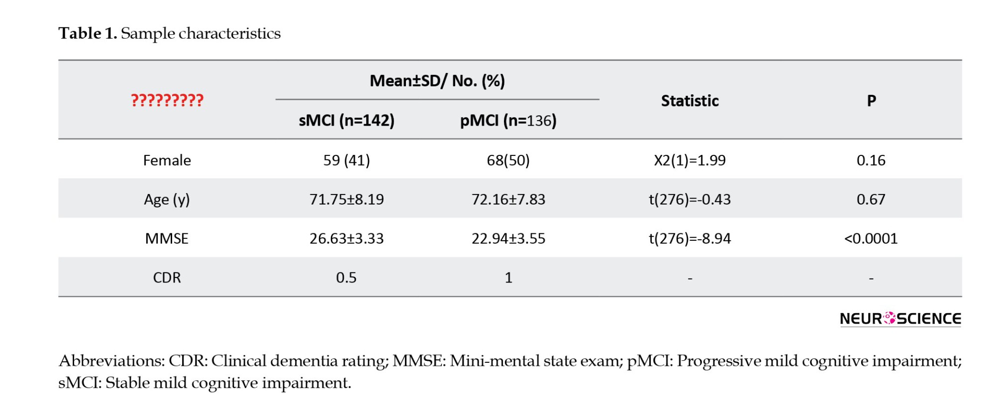
In this study, data from 278 human participants were used. These human participants’ data were extracted from the ADNI (Jack et al., 2008; Jack et al., 2010). Table 1 presents demographic information; the mini-mental state examination (MMSE) is a widely used cognitive measure in clinical and research settings to assess the cognitive status in AD). The data used in this study can be accessed at ADNI data. Other researchers can access these data using the same procedures as the authors. Researchers can access the data by logging into the ADNI website and following these steps: Download > Image collections > Advanced search > Search > Select the scans > Add to collection > CSV download > Advanced download. A complete listing of ADNI investigators can be found at ADNI data. Public access to the database is available. The ADNI was launched in 2003 to test whether serial MRI, fMRI, other biological markers, and clinical and neuropsychological assessments can be combined to measure the progression of MCI and early AD. For this study, we used subjects with at least three years of follow-up diagnosed with MCI at baseline. Participants with stable clinical dementia rating (CDR) scores of 0.5 throughout the follow-up period were classified as having sMCI. Participants with pMCI showed a change in clinical dementia rating (CDR) from 0.5 at baseline to 1 at the final assessment (Zamani et al., 2022). The rs-fMRI data were acquired using a high-field 3 Tesla Philips MRI scanner and an echo-planar imaging sequence. Data for each subject consisted of 140 volumes, each with 48 slices, 3.3 mm slice thickness, spatial resolution of 3×3×3 mm3, flip angle of 80 degrees, 30 ms echo time, and a plane matrix of 64×64. The time between two consecutive volumes was 2s.
Data preprocessing
Resting-state functional magnetic resonance imaging (rs-fMRI) data preprocessing and time series extraction
The preprocessing pipeline for the rs-fMRI data comprised several essential steps to ensure data quality and reliability. The initial five volumes were discarded to mitigate the influence of T1- equilibration effects. Subsequent preprocessing steps encompassed functional realignment and unwarping, correction for slice-timing discrepancies, identification, and handling of outlier volumes to address subject-motion artifacts, direct segmentation, and normalization into the standard Montreal Neurological Institute (MNI) space, and spatial convolution with an 8 mm full-width half-maximum Gaussian kernel for functional smoothing. Low-frequency filtering within the range of 0.01 to 0.1 Hz was applied to retain the relevant fluctuations (Whitfield-Gabrieli & Nieto-Castanon, 2012).
The rs-fMRI data were preprocessed using the CONN toolbox. The Harvard-Oxford Cortical atlas with 136 regions of interest (ROIs) was employed for brain parcellation. For each ROI, a single signal was obtained by averaging the time series of its voxels. The final rs-fMRI data were x ϵ RM×T, where M=136 and T=135 were the numbers of ROIs and time samples, respectively.
Graph frequency bands (GFBs)
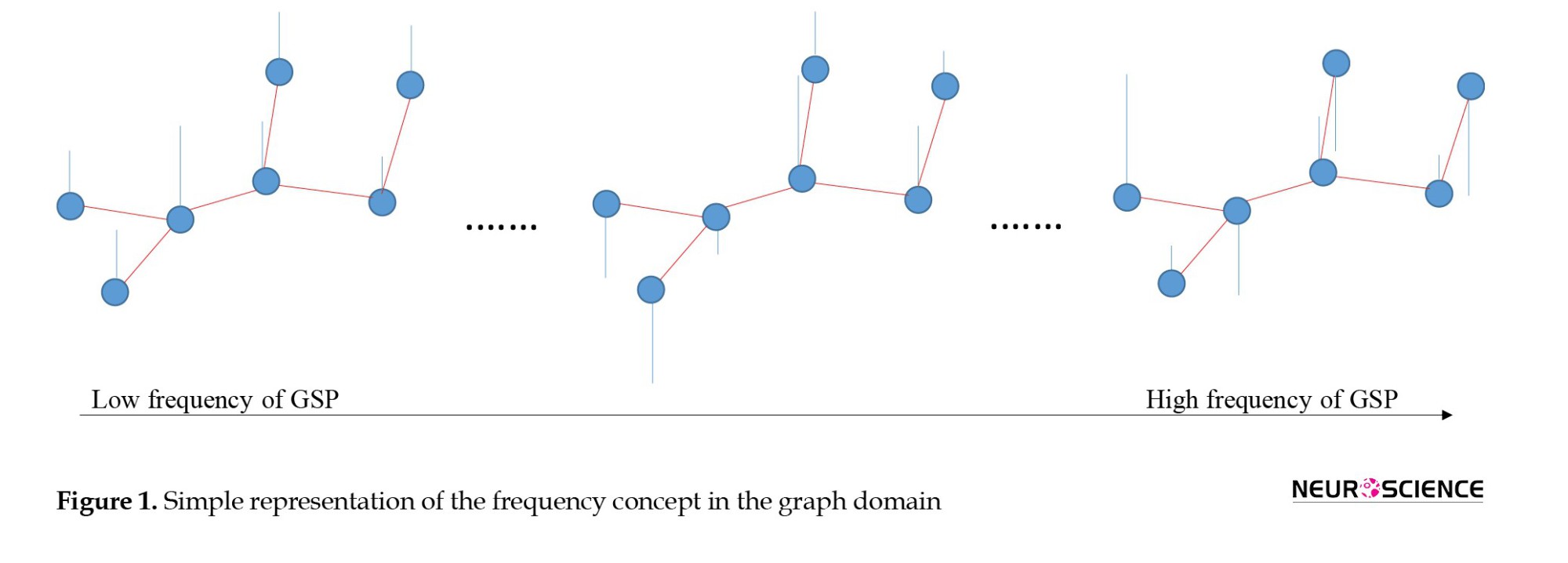
The frequency content of the graph signal is defined according to the signal changes across connected vertices at a given time point. At low frequencies, connected vertices show similar signals (indicating alignment). At high frequencies, the variability of the connected vertices’ signals is high compared to each other (indicating liberality). In liberality, the vertices (brain ROIs) showed less respect for their underlying connectivity structures. By approaching from low frequency to high frequency, the graph signal behavior changes from alignment to liberality (Figure 1).
The graph frequencies are defined using the combinatorial Laplacian matrix L ϵ RN×N (Shuman et al., 2013), as follows:
(1) L=D-A
where A is the adjacency matrix, and D is a diagonal matrix, and its kth diagonal element represents the degree of the kth vertex, i.e. Dkk= ∑Nj=1 Akj. The adjacency matrix of GSP represents its underlying graph. The eigendecomposition of L provides the V and A, which are the eigenvector and diagonal eigenvalues matrices, respectively.
The eigenvectors represent graph frequency modes and are used for GFT. The GFT of brain signal x ϵ R136×135 is obtained as

where 136 and 135 are the number of ROIs and time points and superscript T denotes the transpose operation, respectively. The inverse GFT (IGFT) of x ̃is attained by
In this domain, the signal changes across connected vertices define frequency levels (in the time domain, the signal changes across time points define frequency levels). Consequently, transitioning from lower to higher frequency levels within the graph amplifies the signal changes across connected vertices. The blue circles and red and blue lines represent vertices, edges, and signals, respectively.
Remarkably, the eigenvector associated with the larger eigenvalue exhibits greater variance and can effectively convey higher graph frequencies (Huang et al., 2018). These higher-frequency modes facilitate the conversion of brain signals with increased variance into the graph frequency domain. Conversely, they can also transform higher-frequency information from the frequency domain back into the brain’s topological domain.
The graph signal is amenable to filtering within the frequency domain, followed by an integrated gasification/Fischer-Tropsch (IGFT) to obtain a graph-filtered signal. The graph filtering process can be mathematically formulated as follows:

where G is a diagonal filtering matrix. In this study, a value of 1 was assigned to the diagonal elements corresponding to the desired frequency modes, while the rest of the modes were set to 0.
In this study, the LFB consisted of the first 45 frequency modes, the HFB comprised the last 45 modes, and the MFB was formed by the remaining 46 modes. Using the “(4)”, the rs-fMRI data underwent filtering to generate graphs corresponding to LFB, MFB, and HFB. Subsequently, for each subject, FC matrices were computed within the LFB, MFB, HFB, and FFB. In this study, the data matrices for LFB, MFB, HFB, and FFB were 136 ×135.
Functional connectivity (FC) matrix
FC between ROIs was computed using Pearson correlation and the SW technique. The SW technique was employed to account for the dynamic nature of brain FC. In this approach, a series of windows with a one-TR shift was applied to each ROI time series. Subsequently, an FC matrix was computed for each window. The final correlation value for an ROI-ROI pair was determined as the median of its FC values. The window was created by convolving a rectangle (width=50 TRs) with a Gaussian (σ=3 TRs) (Huang et al., 2018). Each subject’s dataset yielded four FC matrices. These matrices were computed using LFB, MFB, HFB, and FFB rs-fMRI data.
To obtain the adjacency matrix (A) of GSP, the FC matrix of FFB was compared between the sMCI and pMCI groups using the Wilcoxon rank sum test. This process identified statistically significant connections between ROI-ROI. Subsequently, for each subject, these significant ROI-ROI connections from the FFB were retained, while the remaining connections were set to zero. Thus, for each subject, an SFC matrix was computed using the FFB FC and the rank sum test. This matrix served as the adjacency matrix (A) for GSP. It should be noted that the SFC for attaining GSP filters were computed using the training data.
Features
The graph, MST, and triadic interaction metrics were individually computed for each of the four FC matrices. The features for this study were extracted from data from 142 subjects with sMCI and 136 subjects with pMCI. The dimension of each FC matrix was 136×136 for the Harvard-Oxford atlas.
Global metrics of graph
A graph G is defined as a set of vertices V(G) and edges E(G). The connectivity matrix can be represented as a graph, with the ROIs as vertices and the connectivity strengths as edge weights. This modeling approach facilitated the exploration of topological distinctions between ASD and typical control (TC) groups using graph metrics. Subsequently, some of the global graph metrics are outlined below (Fornito et al., 2016).
Global efficiency (GE): The average inverse shortest-path length in the network. In this study, the shortest path between two ROIs is defined as the distance between them.
Mean eccentricity (ME): For each ROI, the eccentricity is equal to the maximum distance between that ROI and the rest of the ROIs. ME equals the average eccentricity of all ROIs.
Radius: The minimum value of eccentricity of all ROIs is equal to the radius.
Diameter: The maximum value of eccentricity of all ROIs is equal to the diameter.
Assortativity coefficient (AC): Each connection involves two ROIs, one initiating and the other terminating it. Let the degrees of the first and second ROIs be as x and y, respectively. Consequently, for all available connections, two vectors, X and Y, are obtained, with the first representing a set of degrees x and the second a set of degrees y. The AC is derived by calculating the correlation coefficient between X and Y. This coefficient ranges between -1 and 1, where positive values indicate that ROIs with similar degrees are more likely to be connected. Conversely, a negative AC value implies that ROIs with larger degrees tend to connect to ROIs with more minor degrees.
Mean of clustering coefficient (MCC): The clustering coefficient is the ratio of triangles around a ROI and ranges between 0 and 1. A value of 1 indicates that connected ROIs to a given ROI are also connected. A lower number of connections in the vicinity of a given ROI results in a decreased clustering coefficient. In this study, the mean clustering coefficient values across all ROIs were calculated for each subject.
Mean of eigenvector centrality (MEC): Connections originating from high-scoring ROIs carry more weight in influencing the score of the ROI under consideration compared to connections from low-scoring ROIs. The EC of an ROI reflects its impact on the network, where an ROI with high EC tends to connect with ROIs that also have high scores. The mean EC across all ROIs was used for each subject in this study.
Mean of strength (MS): The strength of a specific ROI is defined as the sum of the weights of edges adjacent to that ROI. In this study, the mean strength values across all ROIs were calculated for each subject.
Modularity: This metric gauges how effectively a network has been partitioned into groups of ROIs. In a network with high modularity, dense connections are observed within groups, while sparse connections occur between groups of ROIs.
All these metrics were computed using the functions provided by the Brain Connectivity Toolbox (Rubinov & Sporns, 2010).
Metrics of MST
A spanning tree is a subgraph of the original graph that is cycle-free and connects all nodes in the original graph. The MST is a tree with the minimum total weight among all possible spanning trees of the original graph (Van Mieghem & Magdalena, 2005; Lee et al., 2012). In this study, the Single Linkage Dendrogram method was employed for the computation of the MST (Liu et al., 2021). Several metrics related to the MST are delineated (Lee et al., 2012; Liu et al., 2021; Noble, 2006).
Radius and diameter: The minimum and maximum values of eccentricity for all ROIs in the MST correspond to the radius and diameter, respectively.
Maximum degree (Degmax): The degree ki is the number of neighbors for ith ROI in the MST. The maximum of all ROI degrees is considered as Degmax.
Leaf fraction (LF): The fraction of leaf ROIs in the MST, where a leaf ROI is defined as an ROI with a degree of one.
Maximum betweenness centrality (BCmax): The BC of a particular ROI is the fraction of all shortest paths that traverse through that ROI. The maximum ROI BC is considered BCmax.
Hierarchy (TH): The tree hierarchy assesses the balance between large-scale integration in the MST, quantified by the leaf fraction, and the concentration of central nodes, also referred to as hubs, measured through the maximum BC. This metric can be expressed as

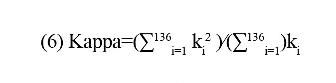
Kappa: This metric quantifies the breadth of the degree distribution. This metric can be formulated as
Metrics of triadic interactions
In this study, as with Moradimanesh and colleagues (Moradimanesh et al., 2021), four types of triads were analyzed in LFB, MFB, HFB, and FFB. These triads were strongly balanced T3: (+ + +), weakly balanced T1: (+ −−), strongly unbalanced T2: (+ + −), and weakly unbalanced T0: (−−−) (Figure 2).
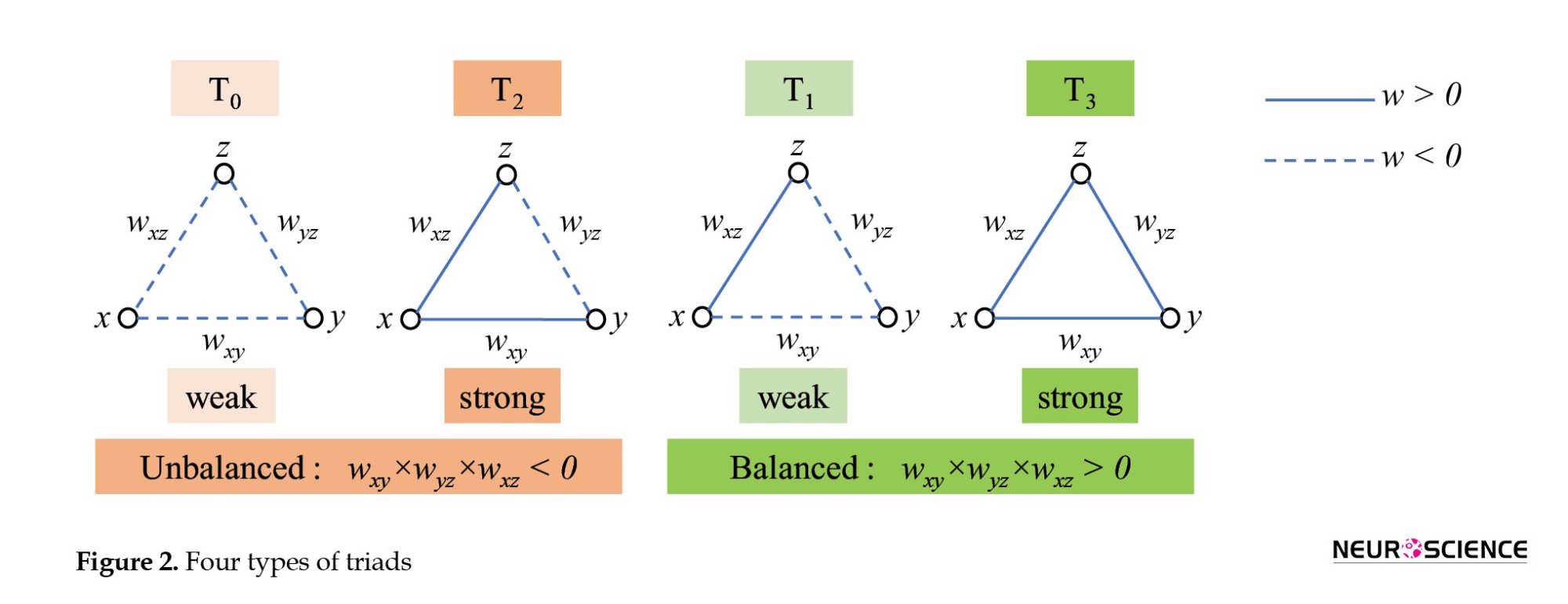
Five metrics were extracted from FC matrices. The first four metrics were the number of the triads T0, T1, T2, and T3. These metrics are also called the triad frequencies (|Ti|, i=0,1,2,3). The fifth one was the energy of the whole-brain network (Un). The Un is defined as
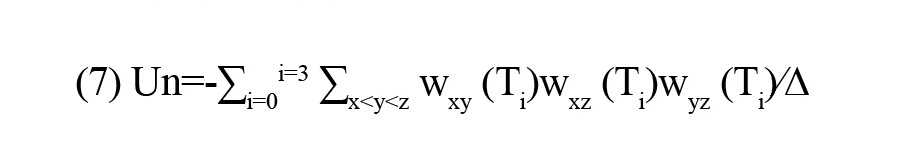
where x, y, and z indicate the ROIs of triad Ti, w is the FC value between ROIs, and ∆ is the total number of triads of the brain.
Tendency to make hub
Hubs are ROIs with a high number of connections and play a pivotal role in the brain network’s topology. In this study, we employed the global hubness metric introduced by Saberi et al. to examine the brain topology of healthy control subjects (Saberi et al., 2021). This metric, named the TMH, is separately defined for positive and negative links as ith and jth:
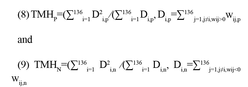
where 136 is the total number of ROIs, Di,p and Di,n represent the positive and negative degrees of ith ROI, respectively, and wij,p and wij,n are the positive and negative weights between ith and jth ROIs.
The subscript of each T denotes the number of positive links.
The TMHP and TMHN demonstrate the network’s propensity to form hubs with positive and negative links, respectively. Therefore, TMH can elucidate the influence of both positive and negative links on the topology of the brain.
The number of links
The number (or occurrence rate) of positive links |P| and negative links |N| are computed for FC matrices of LFB, MFB, HFB, and FFB, separately. By obtaining information on |P| and |N|, it can be determined whether |Ti|s and TMHs may vary between groups, even when there is no difference in the number of positive and negative links.
Feature selection
A total of 100 features were extracted from the four FC matrices (LFB, MFB, HFB, FFB) for each subject. This set included 25 features in each matrix, distributed as follows, graph (9), MST (7), triadic (5), TMH (2), and number of links (2). To improve the efficiency and accuracy of the classification algorithm, feature selection was performed.
Feature selection plays a pivotal role in machine learning by reducing dataset dimensionality and improving classification algorithm performance and accuracy. In this study, we employed two optimization algorithms, PSO and SA, to identify the most informative set of features (Abualigah et al., 2018; Mafarja & Mirjalili., 2017).
PSO is a stochastic optimization technique inspired by the behavior of swarming animals, such as birds and fish. It operates by representing potential solutions as particles that traverse the search space. Particles adjust their positions and velocities based on cognitive and social parameters, and the overall rate of change is regulated by an inertia parameter. Specifically, particles seek optimal regions of the search space through interaction with other particles in the population. For our study, we utilized a swarm size of 20 particles, while setting cognitive and social parameters to 1.5 and inertia to 0.72.
SA employs a probabilistic approach to accept or reject solutions. The algorithm initiates with a randomly generated solution and iteratively generates neighboring solutions based on a predefined neighborhood structure. A fitness function evaluates each generated solution. Improved solutions are accepted, and worse neighbors are accepted probabilistically, governed by the Boltzmann distribition, P=e-θ/ T. In this equation, θ denotes the difference between the fitness of the best solution and the generated neighbor, while T represents a temperature parameter. The temperature T decreases over iterations according to a cooling schedule. In our study, the initial temperature T was set to 10 (Mafarja & Mirjalili., 2017).
By utilizing PSO and SA, we aimed to identify a reduced set of features that significantly contributed to the classification task. This feature selection process not only streamlines the dataset but also enhances the classification performance, making our analysis more effective and efficient. Feature selection was performed within each cross-validation fold to avoid test-set contamination and ensure an unbiased evaluation of predictive performance.
Classification
To discriminate between progressive MCI (pMCI) and stable MCI (sMCI), we employed an SVM with a radial basis function (RBF) kernel. This classification technique was executed using a robust 10-fold cross-validation approach, a well-established practice in machine learning evaluation. The RBF kernel function was chosen for its universal applicability across various sample distributions. It offers flexibility by adjusting parameters to adapt to the data’s inherent characteristics (Noble, 2006).
We employed a comprehensive set of evaluation metrics to assess the classifier’s performance. These metrics include accuracy (Acc.), sensitivity (Sen.), and specificity (Spec.), which provide insight into the classifier’s effectiveness in correctly classifying subjects. The evaluation process involves seperating true labels from the test set, then using utilizing the trained classifier to predict labels on the test set. The parameters are calculated using the following equations:
(10) Accuracy or Acc=
(11) Sensitivity or Sen=
(12) Specificity or Spec=
where TP, FP, TN, and FN represent true positives, false positives, true negatives, and false negatives, respectively. Here, TP stands for true positives, FP for false positives, TN for true negatives, and FN for false negatives. These metrics collectively illuminate the classifier’s ability to distinguish between pMCI and sMCI subjects.
Additionally, receiver operating characteristic (ROC) curves were employed to visually compare the performance of different classifiers. The ROC curve is a graphical representation where the vertical and horizontal axes represent the false-positive and actual-positive rates, respectively. A higher area under the ROC curve indicates better classifier performance, reflecting its capacity to discriminate between the two classes.
The rigorous evaluation process, combining metrics and visualization techniques, provides a comprehensive assessment of the classification model’s accuracy and reliability in identifying subjects with progressive and stable MCI.
Results
This study employed two distinct methodologies to explore the impact of frequency bands and diverse feature types on classification performance, with feature selection performed using both PSO and SA algorithms. Table 2 presents the outcomes of these investigations.
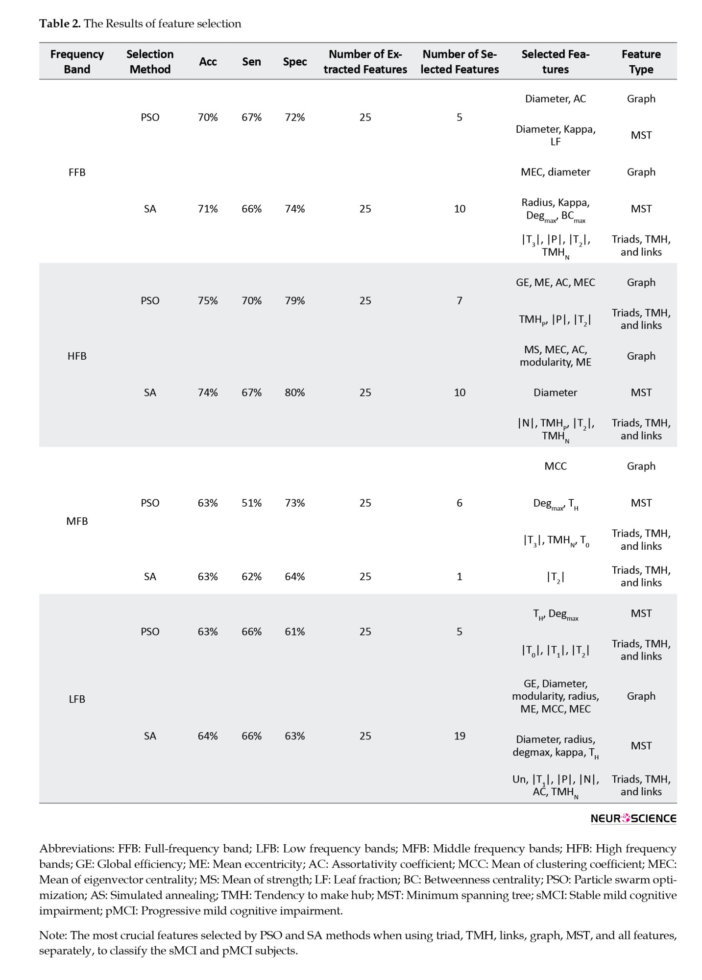
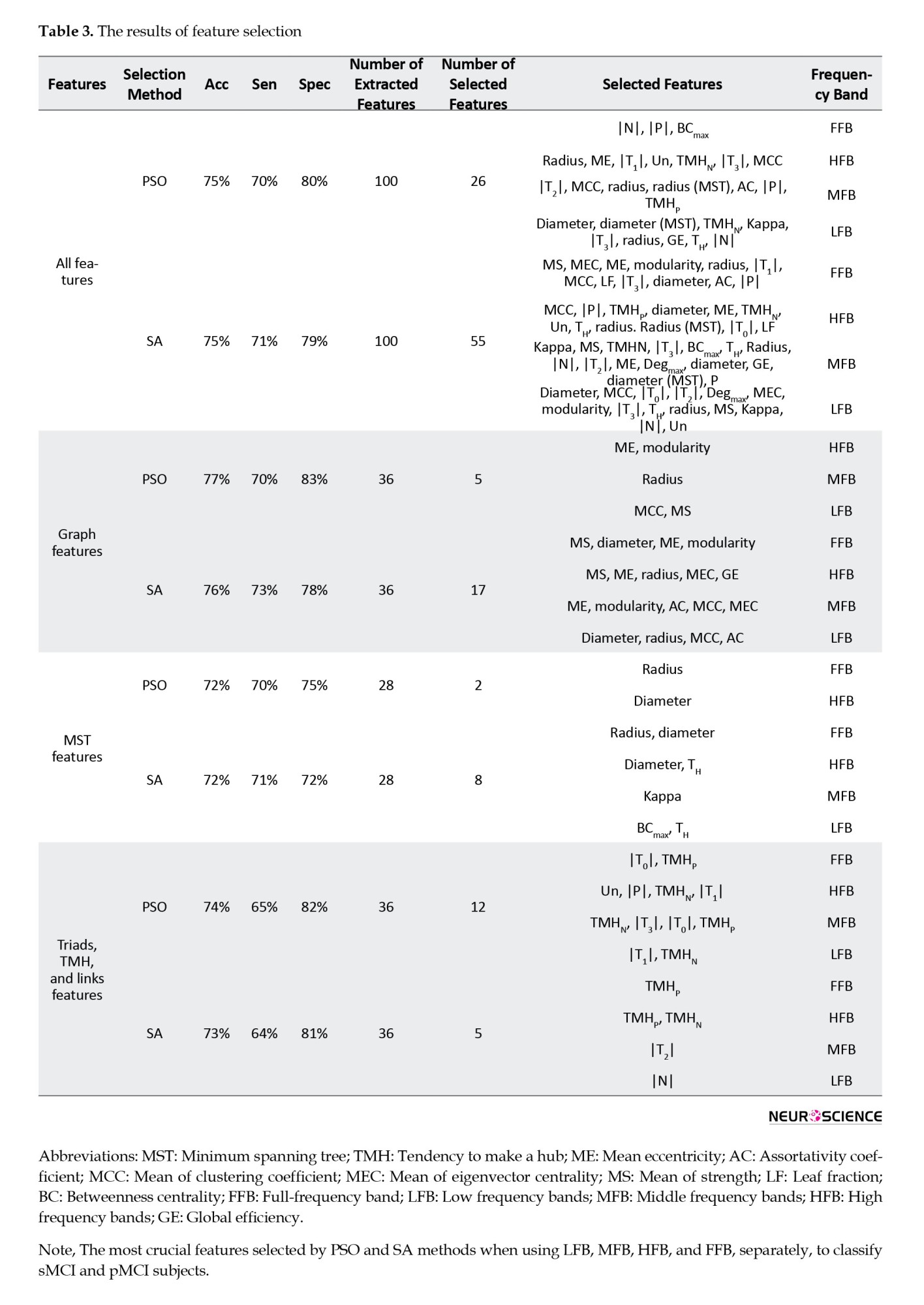
In the first approach, four feature sets were separately used to classify sMCI and pMCI. These groups were all features (100), graph features (36), MST features (28), and triads, TMH, and link features (36) (the number in parentheses indicates the number of features). In this approach, the effect of features over all frequency bands of the graph was studied. The frequency bands were FFB, LFB, MFB, and HFB. In the second approach, features extracted from FFB, LFB, MFB, and HFB were separately used for classification. This analysis could show which frequency bands offered the best and the worst features for classification. For each frequency band, all features of the graph, MST, Triads, TMH, and Links were employed (25 features in total). After feature selection and classification, the results shown in Tables 2 and 3 were obtained for the first and second approaches, respectively.
By reviewing the results in Table 2, it can be observed that the graph-featured offered the highest accuracy for both SA (76%) and PSO (77%) methods. However, the PSO offered 1% and 5% more accuracy and specificity than SA by selecting a much lower number of features (five features) than SA (17 features). The five features, selected by PSO, were (MCC, MS)/radius/(ME, modularity) from LFB/MFB/HFB, respectively. The results with all features were close to those with graph features in terms of accuracy, specificity, and sensitivity. However, this closeness was achieved at the cost of using many more features (26 and 55 for the PSO and SA methods, respectively). The fewest selected features were for MST features when using PSO as the feature selection method. In this case, the radius (in FFB) and diameter (in HFB) features offered 72%, 70%, and 75% of accuracy, sensitivity, and specificity, respectively. The lowest classification performance was obtained by MST features (accuracy of 72%). By reviewing Table 2, it can be observed that PSO, compared to SA, selected much fewer features in many cases while offering similar or better classification performance.
By reviewing the results of the second approach, it is evident that the worst/best classification performance was for the LFB and MFB/HFB features, respectively. The best accuracies in the (LFB and MFB)/HFB were (64% and 63%)/75%, respectively. The best performance in the HFB was achieved using seven features selected by PSO. These seven features were (GE, ME, AC, MEC) of graphs and (TMHP, |P|, |T2|) of triads, TMH and links. The corresponding sensitivity and specificity were 70% and 79%, respectively. In the MFB, an accuracy of 63% was obtained using only one feature (|T2|) selected by SA. Overall, the best classification performance in terms of offering higher accuracy with a lower number of features was achieved using graph features selected by PSO.
Discussion
This study presents a novel approach to classify sMCI and pMCI using a combination of graph frequency bands and functional connectivity-based features extracted from rs-fMRI data. The classification task was facilitated by employing PSO and SA algorithms for feature selection, followed by a SVM with RBF kernel for classification. The proposed method aims to predict the conversion of MCI to AD and offers potential insights into the underlying neurobiological changes associated with disease progression.
The research methodology involved several key steps. First, rs-fMRI data preprocessing was conducted using the CONN toolbox, which included various processing steps to ensure data quality and reliability. FC matrices were computed for the following frequency bands, FFB, LFB, MFB, and HFB. These FC matrices were used to extract a diverse set of features, encompassing global graph metrics, MST metrics, triadic interaction metrics, TMH metrics, and the number of positive and negative links.
The feature selection process played a crucial role in enhancing classification accuracy. Both PSO and SA algorithms were employed to identify the most relevant features for distinguishing between sMCI and pMCI groups. The resulting feature subsets demonstrated distinct patterns depending on the algorithm used and the type of features considered.
The classification performance of the proposed method was evaluated using a SVM with an RBF kernel and a 10-fold cross-validation framework. Significantly, the test data were not utilized in any aspect of feature selection. The results revealed promising accuracy rates, with PSO achieving a 77% accuracy using only five selected features. These findings demonstrated the potential clinical utility of the proposed approach for predicting MCI-to-AD conversion, which could inform treatment plans and clinical trials.
Interpretability emerged as a significant advantage of the proposed method, particularly compared with complex models, such as deep neural networks (DNNs), which often lack transparency. The selected features in this study were based on the connectivity patterns of distinct brain regions, contributing to a better understanding of the underlying neurobiology.
The key findings of the analysis highlighted the importance of specific features in classification. For instance, ME and Modularity of the HFB were found to be particularly altered between patients with sMCI and pMCI, while MCC and MS features of the LFB exhibited strong discriminatory power. Additionally, the radius feature in the MFB was identified as a key contributor to the classification of these two groups.
Comparing to SA, PSO achieved higher accuracy with fewer features. This study underscored the potential of graph analysis of functional connectivity and the effectiveness of the PSO algorithm combined with a simple SVM for accurate classification.
In summary, this study contributes to the field of neuroimaging and cognitive health by presenting a novel approach that combines graph frequency bands, functional connectivity-based features, and advanced feature selection techniques for the classification of stable and progressive MCI. This study addresses the pressing need for early and accurate detection of cognitive decline, particularly in the context of predicting MCI-to-AD conversion.
A notable strength of this study is its innovative approach to feature selection. The PSO and SA algorithms effectively navigate the high-dimensional feature space to identify a subset of features most relevant to accurate classification. This process enhances model performance, simplifies the classification task, and contributes to interpretability. The selected features highlight specific connectivity patterns that differentiate sMCI from pMCI patients, offering valuable insights into the neurobiological underpinnings of disease progression.
The study’s findings highlight the importance of different frequency bands and specific connectivity features for classification. The identification of key features, such as modularity and mean eccentricity in the HFB, mean clustering coefficient and mean strength in the LFB, and radius in the MFB, provides meaningful insights into the altered network properties associated with cognitive decline.
The study’s scope focused on the classification of sMCI and pMCI using rs-fMRI data, and future research could extend this framework to larger and more diverse datasets, encompassing longitudinal data to capture temporal changes in connectivity patterns.
Conclusion
This study presents a comprehensive and innovative method for the early classification of stable and progressive MCI using graph frequency bands and FC-based features. The combination of advanced feature selection techniques and a well-designed classification pipeline demonstrates the potential for accurate prediction of MCI-to-AD conversion. This approach holds promise as a valuable tool for clinicians and researchers seeking to enhance early detection and intervention strategies for neurodegenerative diseases. The continued development and validation of such methodologies have the potential to significantly impact the field of cognitive health and the understanding of neurodegenerative processes.
Ethical Considerations
Compliance with ethical guidelines
All ethical principles were considered in this article. The data used in this study were obtained from the Alzheimer’s Disease Neuroimaging Initiative (ADNI) database. All participants in the ADNI study provided written informed consent at the time of enrollment. Participants were informed about the purpose of the research, the procedures involved, and their right to withdraw from the study at any time. The confidentiality of participants’ information was assured, and all data were fully anonymized. The study procedures were conducted in accordance with the principles of the Declaration of Helsinki.
Funding
The authors declare that no funds, grants, or other support were received during the preparation of this manuscript.
Authors' contributions
All authors contributed equally to the conception and design of the study, data collection and analysis, interception of the results and drafting of the manuscript. Each author approved the final version of the manuscript for submission.
Conflict of interest
The authors declared no conflict of interest.
Acknowledgments
The authors thank the Alzheimer’s Disease Neuroimaging Initiative (ADNI) (National Institutes of Health Grant U01 AG024904) and DOD ADNI (Department of Defense award number W81XWH-12-2-0012) for generously sharing data.
References
Dementia affects approximately 50 million individuals worldwide, with nearly 10 million new cases emerging annually (Peterson et al., 1999). Among dementia subtypes, Alzheimer’s disease (AD) is the most prevalent, accounting for over half of all cases. Amnestic mild cognitive impairment (MCI) occupies a pivotal intermediate stage between healthy controls (HC) and AD. Individuals with MCI face an escalated risk of transitioning to AD, with an approximate annual conversion rate of 15%. Notably, the MCI cohort exhibits significant heterogeneity, with only a subset progressing to AD (Peterson et al., 1999; Petersen et al., 2009). Early-stage intervention for AD is a considerable clinical challenge. Established biomarkers for AD prediction include Aβ accumulation and hyperphosphorylated tau (Spillantini & Goedert, 2013). Traditionally, the verification of amyloid and tau deposits necessitates invasive techniques, such as positron emission tomography (PET) and cerebrospinal fluid (CSF) analysis. Conversely, magnetic resonance imaging (MRI) enables evaluation of neurodegenerative signs, including atrophy and neuronal loss, indicative of amyloid and tau deposition (Bateman et al., 2012).
MRI and resting-state functional MRI (rs-fMRI) have emerged as valuable tools for early-stage clinical assessment of AD and disease progression (Lee et al., 2013). While task-based fMRI examines brain function during cognitive tasks, rs-fMRI captures spontaneous low-frequency brain activity, making it valuable for AD diagnosis (Lee et al., 2013; Khazaee et al., 2015). In conventional functional connectivity (FC) analyses, brain region correlations are assumed to remain constant throughout an imaging session. Dynamic FC, a more recent extension of traditional FC, captures evolving interactions and is considered a more accurate representation of functional brain networks (Khazaee et al., 2015; Allen et al., 2014). It is important to note that neuroimaging techniques are currently predominantly used as research tools for AD diagnosis.
Robust biomarker identification is pivotal for distinguishing progressive MCI (pMCI) from stable MCI (sMCI), facilitating early AD diagnosis and treatment. PMCI refers to individuals with MCI who exhibit continuous cognitive function decline, ultimately progressing to AD. SMCI refers to individuals whose cognitive impairment does not significantly worsen over time, remaining stable without advancing to AD. Recent studies have integrated multimodal biomarkers, including PET and rs-fMRI, with machine learning algorithms to predict the conversion from MCI to AD (Chang & Glover, 2010; Hinrichs et al., 2011; Young et al., 2013; Liu et al., 2013; Zamani et al; 2022). Notably, functional neuroimaging holds greater promise for early AD detection compared to structural neuroimaging (Yassa et al., 2010; Sperling, 2011; Wierenga & Bondi, 2007). Functional MRI, which evaluates brain function during cognitive tasks, demonstrates remarkable sensitivity to early disease processes, often preceding observable impairments in standard neuropsychological tests (Pievani et al., 2011; Teipel et al., 2015). Conversely, rs-fMRI captures spontaneous fluctuations in brain activity, making it less dependent on individual cognitive capabilities (Shakil et al., 2016; Vemuri et al., 2012; Fox & Greicius, 2010).
A key attribute of rs-fMRI’s is its capacity to assess FC alterations (Greicius et al., 2003; Sheline & Raichle., 2013), a prevalent hallmark of AD (Zhang et al., 2010; Zhou et al., 2010; Dennis & Thompson, 2014; Jalilianhasanpour et al., 2019). Studies have shown that cognitive impairment severity correlates with increasing disruptions in connectivity patterns, suggesting that FC changes are potential biomarkers of cognitive dysfunction in MCI. Importantly, longitudinal FC alterations are more pronounced in the early stages of AD (Zhan et al., 2016). FC analysis inherently involves network interactions, making graph theory an effective tool for investigating global and local brain region characteristics (Bullmore & Sporns, 2009; Bullmore & Sporns, 2010; Heuvel & Sporns, 2013; Farahani et al., 2019). This approach has successfully elucidated insights into various neurological conditions, including depression, Parkinson’s disease, and AD. This method has been successfully used in a wide range of applications in both healthy participants and patients (Blanken et al., 2021), such as depression (Yun & Kim, 2021; Amiri et al., 2021), Parkinson’s disease (Beheshti & Ko, 2021), and AD (Dai et al., 2021). Graph theory, a powerful topological tool, allows for novel investigation of AD (Dai et al., 2021; Tijms et al., 2013; Brier et al., 2014; He & Evans, 2010). It enables us to compare the brain network organization between patients and healthy individuals (Bassett & Bullmore, 2009; Stam, 2014) and, importantly, provides insights into how these networks change across different stages of the disease (Hojjati et al., 2017; Khazaee et al., 2017). This method delves deeper, not only identifying brain differences but also revealing compensatory mechanisms that might explain why some individuals with similar cognitive scores exhibit different brain activity patterns (Behfar et al., 2020; Gregory et al., 2017; Yao et al., 2010; Cabeza et al., 2018).
Graph-theoretic methods, such as the minimum spanning tree (MST), provide valuable insights into brain connectivity. In this context, nodes represent brain regions, and edges represent functional connections (weights) between them. The MST is a subgraph that connects all nodes with the minimum possible total edge weight, avoiding cycles and redundant connections. This simplification retains the essential network structure, offering an “impartial” representation by focusing on the most critical connections. This impartial technique significantly streamlines the network structure while retaining its essential framework. Notably, this ensures the network’s neurological interpretability, making it a widely employed tool in neuroimaging (Guo et al., 2017; van Dellen et al., 2018). Using this method, the edges in the network are simplified, ensuring that the selected spanning tree has the smallest possible weight.
While most brain network analyses focus on pairwise interactions between regions, the complex reality of the human brain suggests higher-order interactions play a crucial role. Investigating higher-order interactions within the brain network can lead to groundbreaking discoveries related to brain function and dysfunction, disease progression, and potentially, treatment development. Moradimanesh and colleagues (Moradimanesh et al., 2021) delved deeper into brain network analysis by examining triadic interactions, involving three interconnected regions. This method allowed them to compare the interaction patterns between individuals with autism spectrum disorder (ASD) and HC. Pearson’s correlation was used as their tool to measure the interaction between regions. The authors explored four distinct triadic interaction patterns, each with specific configurations of positive and negative FC values (+ and −). These triads were strongly balanced T3: (+ + +), strongly unbalanced T2: (+ + −), weakly balanced T1: (+ − −), and weakly unbalanced T0, (− − −). The study revealed that balanced brain interactions were more common in both the ASD and HC groups, while unbalanced interactions were less frequent. Additionally, the energy levels of the salience network (SN) and the default mode network (DMN) were found to be lower in patients with AD, suggesting potential challenges in adapting behavior. In another study of triadic interactions, Saberi et al. introduced the metrics of the tendency to make hub (TMH). They showed that negative links of the resting-state network make hubs to reduce balance-energy and push the network into a more stable state compared to null-networks with trivial topologies (Saberi et al., 2021).
Graph signal processing (GSP) is a recently developed field that analyzes brain activity through a unique lens called the topological frequency (Shuman et al., 2013; Ortega et al., 2018; Jafadideh & Asl, 2022; Jafadideh & Asl, 2022). This approach relies on two key elements, A graph representing brain connections and brain activity mapped onto that graph. Using a tool called the graph Fourier transform (GFT), GSP can compute different topological frequency filters and identify different patterns hidden within these connections. Excitingly, recent research has shown that GSP can be used to diagnose early-stage MCI based on brain activity data from two independent studies (Padole, 2021; Fan et al., 2008).
Early diagnosis of AD at the MCI stage is vital for developing effective treatments. However, the heterogeneity of AD has made early diagnosis challenging. Many machine learning algorithms have been applied to the diagnosis of MCI and to the prediction of MCI-to-AD conversion (Cabral et al., 2015; Blum & Langley, 1997). Given the large number of extracted features from neuroimaging data, feature selection is essential before classification. Modern machine learning methods often incorporate implicit feature-selection mechanisms. While explicit feature selection as a preprocessing step is less common, it remains beneficial for reducing dataset dimensionality and improving classification accuracy. By performing this step, the most representative optimal feature set is selected, and the redundant features for diagnosing AD progression are neglected (Reunanen, 2003; John et al., 1994). High-efficacy feature selection algorithms are useful to speed up the diagnostic system and enhance its diagnostic performance. The performance of feature selection and classification methods depends on hyperparameter tuning and the specific characteristics of the dataset. Effective optimization requires careful consideration of these parameters to achieve robust results. Feature selection is particularly complicated due to the nonlinear nature of classification methods, more parameters do not necessarily lead to better performance, and parameter dependencies are common. Therefore, it is essential to utilize a suitable optimization method that can handle high-dimensional, nonlinear search spaces (Chu et al., 2012; Bicacro et al., 2012).
In this study, the topological filters were obtained through the GFT tool and SFCmatrix. Each subject had a unique SFC matrix, computed using Pearson correlation and the Wilcoxon rank sum-test (Mann & Whitney., 1947). The GFT was used to compute three topological frequency filters, which were then used to separate the brain activity data (rs-fMRI) into three distinct frequency bands, low (LFB), middle (MFB), and high (HFB). FC matrices were computed for each frequency band using the filtered data. Additionally, an FC matrix was computed for the unfiltered data, termed the full-frequency band (FFB). Some graph global metrics, MST metrics, triadic interaction metrics, TMH metrics, and the number of positive and negative links were computed from the LFB, MFB, HFB, and FFB FC matrices. To identify the most important features, feature selection was performed using particle swarm optimization (PSO) and simulated annealing (SA) (Abualigah, 2018; Mafarja & Mirjalili, 2017). Subsequently, the selected features were used to classify AD and MCI. Our analysis achieved higher accuracy compared to several prior methods. Specifically, Raamana et al. (2015) constructed a brain network based on cortical thickness differences and utilized a multi-core Bayesian classifier, achieving 64% classification accuracy for distinguishing pMCI from sMCI (Raamana, 2015). Similarly, Wei et al. (2016) proposed a classification framework incorporating MRI and network features, achieving an accuracy of 76% (Wei et al., 2016). Liu and colleageus developed a multi-modal classification method combining PET and MRI data, achieving an accuracy of 67% (Liu et al., 2014). Binbin Fu et al. (2025) introduced a multi-modal deep domain adaptation (MM-DDA) model that integrates MRI and PET data. Their model achieved 81.81% accuracy in distinguishing pMCI from sMCI (Fu et al., 2025).
Hu et al. (2025) proposed MME-TransENet, a novel hybrid convolutional neural network (CNN)-transformer architecture designed to capture fine-grained and spatiotemporal features from MRI to predict MCI progression. Evaluated on the AD Neuroimaging Initiative (ADNI) dataset, MME-TransENet achieved state-of-the-art performance with an accuracy of 84.74% (Hu et al., 2025). Zhang and colleageus introduced a similar graph-theoretic and machine-learning framework that integrated cortical thickness features, structural brain networks, and sub-frequency rs-fMRI network metrics. In their study, the combination of the random subset feature selection algorithm (RSFS) with a support vector machine (SVM) classifier yielded the best classification performance, achieving accuracies of 84.7% for MCI converters (MCIc) versus non-converters (MCInc) and 89.8% for MCI converters (MCIc) versus AD (Zhang et al., 2021). Karim and colleagues applied machine learning and graph theory to resting-state fMRI data to predict AD. Using 5-fold cross-validation, their models achieved high accuracy, with the SVM performing at approximately 82%. These findings align with previous research and support the use of machine learning and graph theory applied to fMRI data for improving early diagnosis of AD (Karim et al., 2024). Minami and colleagues proposed a preprocessing method for resting-state fMRI data that includes principal component analysis, window-based functional connectivity analysis, and hypothesis-based feature selection. Using a machine learning model to classify cognitively normal and MCI groups, their approach achieved the highest performance with a fivefold cross-validation accuracy of 84.7%, recall of 67.0%, precision of 63.5%, and F1 score of 63.3% (Minami et al., 2025). The strong alignment between our results and theirs underscores the robustness and reliability of conventional machine learning models paired with carefully selected neuroimaging features, especially in studies with limited sample sizes where deep learning methods may underperform. Our approach, which relies on a limited number of fMRI features, results in lower computational complexity than multi-modality data approaches. Our analysis provides FC-based features that are easy to interpret and understand.
The reminder of this study is organized as follows: Section 2 describes the dataset, preprocessing methods,Brain parcellation, FC, graph frequency bands, studied features, feature selection, and classification. The subsequent section, results, presents the outcomes of the feature selection and classification processes. Finally, the following two sections discuss the results and present the concluding remarks and insights.
Materials and Methods
Participants and data acquisition
In this study, data from 278 human participants were used. These human participants’ data were extracted from the ADNI (Jack et al., 2008; Jack et al., 2010). Table 1 presents demographic information; the mini-mental state examination (MMSE) is a widely used cognitive measure in clinical and research settings to assess the cognitive status in AD). The data used in this study can be accessed at ADNI data. Other researchers can access these data using the same procedures as the authors. Researchers can access the data by logging into the ADNI website and following these steps: Download > Image collections > Advanced search > Search > Select the scans > Add to collection > CSV download > Advanced download. A complete listing of ADNI investigators can be found at ADNI data. Public access to the database is available. The ADNI was launched in 2003 to test whether serial MRI, fMRI, other biological markers, and clinical and neuropsychological assessments can be combined to measure the progression of MCI and early AD. For this study, we used subjects with at least three years of follow-up diagnosed with MCI at baseline. Participants with stable clinical dementia rating (CDR) scores of 0.5 throughout the follow-up period were classified as having sMCI. Participants with pMCI showed a change in clinical dementia rating (CDR) from 0.5 at baseline to 1 at the final assessment (Zamani et al., 2022). The rs-fMRI data were acquired using a high-field 3 Tesla Philips MRI scanner and an echo-planar imaging sequence. Data for each subject consisted of 140 volumes, each with 48 slices, 3.3 mm slice thickness, spatial resolution of 3×3×3 mm3, flip angle of 80 degrees, 30 ms echo time, and a plane matrix of 64×64. The time between two consecutive volumes was 2s.
Data preprocessing
Resting-state functional magnetic resonance imaging (rs-fMRI) data preprocessing and time series extraction
The preprocessing pipeline for the rs-fMRI data comprised several essential steps to ensure data quality and reliability. The initial five volumes were discarded to mitigate the influence of T1- equilibration effects. Subsequent preprocessing steps encompassed functional realignment and unwarping, correction for slice-timing discrepancies, identification, and handling of outlier volumes to address subject-motion artifacts, direct segmentation, and normalization into the standard Montreal Neurological Institute (MNI) space, and spatial convolution with an 8 mm full-width half-maximum Gaussian kernel for functional smoothing. Low-frequency filtering within the range of 0.01 to 0.1 Hz was applied to retain the relevant fluctuations (Whitfield-Gabrieli & Nieto-Castanon, 2012).
The rs-fMRI data were preprocessed using the CONN toolbox. The Harvard-Oxford Cortical atlas with 136 regions of interest (ROIs) was employed for brain parcellation. For each ROI, a single signal was obtained by averaging the time series of its voxels. The final rs-fMRI data were x ϵ RM×T, where M=136 and T=135 were the numbers of ROIs and time samples, respectively.
Graph frequency bands (GFBs)
The frequency content of the graph signal is defined according to the signal changes across connected vertices at a given time point. At low frequencies, connected vertices show similar signals (indicating alignment). At high frequencies, the variability of the connected vertices’ signals is high compared to each other (indicating liberality). In liberality, the vertices (brain ROIs) showed less respect for their underlying connectivity structures. By approaching from low frequency to high frequency, the graph signal behavior changes from alignment to liberality (Figure 1).
The graph frequencies are defined using the combinatorial Laplacian matrix L ϵ RN×N (Shuman et al., 2013), as follows:
(1) L=D-A
where A is the adjacency matrix, and D is a diagonal matrix, and its kth diagonal element represents the degree of the kth vertex, i.e. Dkk= ∑Nj=1 Akj. The adjacency matrix of GSP represents its underlying graph. The eigendecomposition of L provides the V and A, which are the eigenvector and diagonal eigenvalues matrices, respectively.
The eigenvectors represent graph frequency modes and are used for GFT. The GFT of brain signal x ϵ R136×135 is obtained as
where 136 and 135 are the number of ROIs and time points and superscript T denotes the transpose operation, respectively. The inverse GFT (IGFT) of x ̃is attained by
In this domain, the signal changes across connected vertices define frequency levels (in the time domain, the signal changes across time points define frequency levels). Consequently, transitioning from lower to higher frequency levels within the graph amplifies the signal changes across connected vertices. The blue circles and red and blue lines represent vertices, edges, and signals, respectively.
Remarkably, the eigenvector associated with the larger eigenvalue exhibits greater variance and can effectively convey higher graph frequencies (Huang et al., 2018). These higher-frequency modes facilitate the conversion of brain signals with increased variance into the graph frequency domain. Conversely, they can also transform higher-frequency information from the frequency domain back into the brain’s topological domain.
The graph signal is amenable to filtering within the frequency domain, followed by an integrated gasification/Fischer-Tropsch (IGFT) to obtain a graph-filtered signal. The graph filtering process can be mathematically formulated as follows:
where G is a diagonal filtering matrix. In this study, a value of 1 was assigned to the diagonal elements corresponding to the desired frequency modes, while the rest of the modes were set to 0.
In this study, the LFB consisted of the first 45 frequency modes, the HFB comprised the last 45 modes, and the MFB was formed by the remaining 46 modes. Using the “(4)”, the rs-fMRI data underwent filtering to generate graphs corresponding to LFB, MFB, and HFB. Subsequently, for each subject, FC matrices were computed within the LFB, MFB, HFB, and FFB. In this study, the data matrices for LFB, MFB, HFB, and FFB were 136 ×135.
Functional connectivity (FC) matrix
FC between ROIs was computed using Pearson correlation and the SW technique. The SW technique was employed to account for the dynamic nature of brain FC. In this approach, a series of windows with a one-TR shift was applied to each ROI time series. Subsequently, an FC matrix was computed for each window. The final correlation value for an ROI-ROI pair was determined as the median of its FC values. The window was created by convolving a rectangle (width=50 TRs) with a Gaussian (σ=3 TRs) (Huang et al., 2018). Each subject’s dataset yielded four FC matrices. These matrices were computed using LFB, MFB, HFB, and FFB rs-fMRI data.
To obtain the adjacency matrix (A) of GSP, the FC matrix of FFB was compared between the sMCI and pMCI groups using the Wilcoxon rank sum test. This process identified statistically significant connections between ROI-ROI. Subsequently, for each subject, these significant ROI-ROI connections from the FFB were retained, while the remaining connections were set to zero. Thus, for each subject, an SFC matrix was computed using the FFB FC and the rank sum test. This matrix served as the adjacency matrix (A) for GSP. It should be noted that the SFC for attaining GSP filters were computed using the training data.
Features
The graph, MST, and triadic interaction metrics were individually computed for each of the four FC matrices. The features for this study were extracted from data from 142 subjects with sMCI and 136 subjects with pMCI. The dimension of each FC matrix was 136×136 for the Harvard-Oxford atlas.
Global metrics of graph
A graph G is defined as a set of vertices V(G) and edges E(G). The connectivity matrix can be represented as a graph, with the ROIs as vertices and the connectivity strengths as edge weights. This modeling approach facilitated the exploration of topological distinctions between ASD and typical control (TC) groups using graph metrics. Subsequently, some of the global graph metrics are outlined below (Fornito et al., 2016).
Global efficiency (GE): The average inverse shortest-path length in the network. In this study, the shortest path between two ROIs is defined as the distance between them.
Mean eccentricity (ME): For each ROI, the eccentricity is equal to the maximum distance between that ROI and the rest of the ROIs. ME equals the average eccentricity of all ROIs.
Radius: The minimum value of eccentricity of all ROIs is equal to the radius.
Diameter: The maximum value of eccentricity of all ROIs is equal to the diameter.
Assortativity coefficient (AC): Each connection involves two ROIs, one initiating and the other terminating it. Let the degrees of the first and second ROIs be as x and y, respectively. Consequently, for all available connections, two vectors, X and Y, are obtained, with the first representing a set of degrees x and the second a set of degrees y. The AC is derived by calculating the correlation coefficient between X and Y. This coefficient ranges between -1 and 1, where positive values indicate that ROIs with similar degrees are more likely to be connected. Conversely, a negative AC value implies that ROIs with larger degrees tend to connect to ROIs with more minor degrees.
Mean of clustering coefficient (MCC): The clustering coefficient is the ratio of triangles around a ROI and ranges between 0 and 1. A value of 1 indicates that connected ROIs to a given ROI are also connected. A lower number of connections in the vicinity of a given ROI results in a decreased clustering coefficient. In this study, the mean clustering coefficient values across all ROIs were calculated for each subject.
Mean of eigenvector centrality (MEC): Connections originating from high-scoring ROIs carry more weight in influencing the score of the ROI under consideration compared to connections from low-scoring ROIs. The EC of an ROI reflects its impact on the network, where an ROI with high EC tends to connect with ROIs that also have high scores. The mean EC across all ROIs was used for each subject in this study.
Mean of strength (MS): The strength of a specific ROI is defined as the sum of the weights of edges adjacent to that ROI. In this study, the mean strength values across all ROIs were calculated for each subject.
Modularity: This metric gauges how effectively a network has been partitioned into groups of ROIs. In a network with high modularity, dense connections are observed within groups, while sparse connections occur between groups of ROIs.
All these metrics were computed using the functions provided by the Brain Connectivity Toolbox (Rubinov & Sporns, 2010).
Metrics of MST
A spanning tree is a subgraph of the original graph that is cycle-free and connects all nodes in the original graph. The MST is a tree with the minimum total weight among all possible spanning trees of the original graph (Van Mieghem & Magdalena, 2005; Lee et al., 2012). In this study, the Single Linkage Dendrogram method was employed for the computation of the MST (Liu et al., 2021). Several metrics related to the MST are delineated (Lee et al., 2012; Liu et al., 2021; Noble, 2006).
Radius and diameter: The minimum and maximum values of eccentricity for all ROIs in the MST correspond to the radius and diameter, respectively.
Maximum degree (Degmax): The degree ki is the number of neighbors for ith ROI in the MST. The maximum of all ROI degrees is considered as Degmax.
Leaf fraction (LF): The fraction of leaf ROIs in the MST, where a leaf ROI is defined as an ROI with a degree of one.
Maximum betweenness centrality (BCmax): The BC of a particular ROI is the fraction of all shortest paths that traverse through that ROI. The maximum ROI BC is considered BCmax.
Hierarchy (TH): The tree hierarchy assesses the balance between large-scale integration in the MST, quantified by the leaf fraction, and the concentration of central nodes, also referred to as hubs, measured through the maximum BC. This metric can be expressed as
Kappa: This metric quantifies the breadth of the degree distribution. This metric can be formulated as
Metrics of triadic interactions
In this study, as with Moradimanesh and colleagues (Moradimanesh et al., 2021), four types of triads were analyzed in LFB, MFB, HFB, and FFB. These triads were strongly balanced T3: (+ + +), weakly balanced T1: (+ −−), strongly unbalanced T2: (+ + −), and weakly unbalanced T0: (−−−) (Figure 2).
Five metrics were extracted from FC matrices. The first four metrics were the number of the triads T0, T1, T2, and T3. These metrics are also called the triad frequencies (|Ti|, i=0,1,2,3). The fifth one was the energy of the whole-brain network (Un). The Un is defined as
where x, y, and z indicate the ROIs of triad Ti, w is the FC value between ROIs, and ∆ is the total number of triads of the brain.
Tendency to make hub
Hubs are ROIs with a high number of connections and play a pivotal role in the brain network’s topology. In this study, we employed the global hubness metric introduced by Saberi et al. to examine the brain topology of healthy control subjects (Saberi et al., 2021). This metric, named the TMH, is separately defined for positive and negative links as ith and jth:
where 136 is the total number of ROIs, Di,p and Di,n represent the positive and negative degrees of ith ROI, respectively, and wij,p and wij,n are the positive and negative weights between ith and jth ROIs.
The subscript of each T denotes the number of positive links.
The TMHP and TMHN demonstrate the network’s propensity to form hubs with positive and negative links, respectively. Therefore, TMH can elucidate the influence of both positive and negative links on the topology of the brain.
The number of links
The number (or occurrence rate) of positive links |P| and negative links |N| are computed for FC matrices of LFB, MFB, HFB, and FFB, separately. By obtaining information on |P| and |N|, it can be determined whether |Ti|s and TMHs may vary between groups, even when there is no difference in the number of positive and negative links.
Feature selection
A total of 100 features were extracted from the four FC matrices (LFB, MFB, HFB, FFB) for each subject. This set included 25 features in each matrix, distributed as follows, graph (9), MST (7), triadic (5), TMH (2), and number of links (2). To improve the efficiency and accuracy of the classification algorithm, feature selection was performed.
Feature selection plays a pivotal role in machine learning by reducing dataset dimensionality and improving classification algorithm performance and accuracy. In this study, we employed two optimization algorithms, PSO and SA, to identify the most informative set of features (Abualigah et al., 2018; Mafarja & Mirjalili., 2017).
PSO is a stochastic optimization technique inspired by the behavior of swarming animals, such as birds and fish. It operates by representing potential solutions as particles that traverse the search space. Particles adjust their positions and velocities based on cognitive and social parameters, and the overall rate of change is regulated by an inertia parameter. Specifically, particles seek optimal regions of the search space through interaction with other particles in the population. For our study, we utilized a swarm size of 20 particles, while setting cognitive and social parameters to 1.5 and inertia to 0.72.
SA employs a probabilistic approach to accept or reject solutions. The algorithm initiates with a randomly generated solution and iteratively generates neighboring solutions based on a predefined neighborhood structure. A fitness function evaluates each generated solution. Improved solutions are accepted, and worse neighbors are accepted probabilistically, governed by the Boltzmann distribition, P=e-θ/ T. In this equation, θ denotes the difference between the fitness of the best solution and the generated neighbor, while T represents a temperature parameter. The temperature T decreases over iterations according to a cooling schedule. In our study, the initial temperature T was set to 10 (Mafarja & Mirjalili., 2017).
By utilizing PSO and SA, we aimed to identify a reduced set of features that significantly contributed to the classification task. This feature selection process not only streamlines the dataset but also enhances the classification performance, making our analysis more effective and efficient. Feature selection was performed within each cross-validation fold to avoid test-set contamination and ensure an unbiased evaluation of predictive performance.
Classification
To discriminate between progressive MCI (pMCI) and stable MCI (sMCI), we employed an SVM with a radial basis function (RBF) kernel. This classification technique was executed using a robust 10-fold cross-validation approach, a well-established practice in machine learning evaluation. The RBF kernel function was chosen for its universal applicability across various sample distributions. It offers flexibility by adjusting parameters to adapt to the data’s inherent characteristics (Noble, 2006).
We employed a comprehensive set of evaluation metrics to assess the classifier’s performance. These metrics include accuracy (Acc.), sensitivity (Sen.), and specificity (Spec.), which provide insight into the classifier’s effectiveness in correctly classifying subjects. The evaluation process involves seperating true labels from the test set, then using utilizing the trained classifier to predict labels on the test set. The parameters are calculated using the following equations:
(10) Accuracy or Acc=
(11) Sensitivity or Sen=
(12) Specificity or Spec=
where TP, FP, TN, and FN represent true positives, false positives, true negatives, and false negatives, respectively. Here, TP stands for true positives, FP for false positives, TN for true negatives, and FN for false negatives. These metrics collectively illuminate the classifier’s ability to distinguish between pMCI and sMCI subjects.
Additionally, receiver operating characteristic (ROC) curves were employed to visually compare the performance of different classifiers. The ROC curve is a graphical representation where the vertical and horizontal axes represent the false-positive and actual-positive rates, respectively. A higher area under the ROC curve indicates better classifier performance, reflecting its capacity to discriminate between the two classes.
The rigorous evaluation process, combining metrics and visualization techniques, provides a comprehensive assessment of the classification model’s accuracy and reliability in identifying subjects with progressive and stable MCI.
Results
This study employed two distinct methodologies to explore the impact of frequency bands and diverse feature types on classification performance, with feature selection performed using both PSO and SA algorithms. Table 2 presents the outcomes of these investigations.
In the first approach, four feature sets were separately used to classify sMCI and pMCI. These groups were all features (100), graph features (36), MST features (28), and triads, TMH, and link features (36) (the number in parentheses indicates the number of features). In this approach, the effect of features over all frequency bands of the graph was studied. The frequency bands were FFB, LFB, MFB, and HFB. In the second approach, features extracted from FFB, LFB, MFB, and HFB were separately used for classification. This analysis could show which frequency bands offered the best and the worst features for classification. For each frequency band, all features of the graph, MST, Triads, TMH, and Links were employed (25 features in total). After feature selection and classification, the results shown in Tables 2 and 3 were obtained for the first and second approaches, respectively.
By reviewing the results in Table 2, it can be observed that the graph-featured offered the highest accuracy for both SA (76%) and PSO (77%) methods. However, the PSO offered 1% and 5% more accuracy and specificity than SA by selecting a much lower number of features (five features) than SA (17 features). The five features, selected by PSO, were (MCC, MS)/radius/(ME, modularity) from LFB/MFB/HFB, respectively. The results with all features were close to those with graph features in terms of accuracy, specificity, and sensitivity. However, this closeness was achieved at the cost of using many more features (26 and 55 for the PSO and SA methods, respectively). The fewest selected features were for MST features when using PSO as the feature selection method. In this case, the radius (in FFB) and diameter (in HFB) features offered 72%, 70%, and 75% of accuracy, sensitivity, and specificity, respectively. The lowest classification performance was obtained by MST features (accuracy of 72%). By reviewing Table 2, it can be observed that PSO, compared to SA, selected much fewer features in many cases while offering similar or better classification performance.
By reviewing the results of the second approach, it is evident that the worst/best classification performance was for the LFB and MFB/HFB features, respectively. The best accuracies in the (LFB and MFB)/HFB were (64% and 63%)/75%, respectively. The best performance in the HFB was achieved using seven features selected by PSO. These seven features were (GE, ME, AC, MEC) of graphs and (TMHP, |P|, |T2|) of triads, TMH and links. The corresponding sensitivity and specificity were 70% and 79%, respectively. In the MFB, an accuracy of 63% was obtained using only one feature (|T2|) selected by SA. Overall, the best classification performance in terms of offering higher accuracy with a lower number of features was achieved using graph features selected by PSO.
Discussion
This study presents a novel approach to classify sMCI and pMCI using a combination of graph frequency bands and functional connectivity-based features extracted from rs-fMRI data. The classification task was facilitated by employing PSO and SA algorithms for feature selection, followed by a SVM with RBF kernel for classification. The proposed method aims to predict the conversion of MCI to AD and offers potential insights into the underlying neurobiological changes associated with disease progression.
The research methodology involved several key steps. First, rs-fMRI data preprocessing was conducted using the CONN toolbox, which included various processing steps to ensure data quality and reliability. FC matrices were computed for the following frequency bands, FFB, LFB, MFB, and HFB. These FC matrices were used to extract a diverse set of features, encompassing global graph metrics, MST metrics, triadic interaction metrics, TMH metrics, and the number of positive and negative links.
The feature selection process played a crucial role in enhancing classification accuracy. Both PSO and SA algorithms were employed to identify the most relevant features for distinguishing between sMCI and pMCI groups. The resulting feature subsets demonstrated distinct patterns depending on the algorithm used and the type of features considered.
The classification performance of the proposed method was evaluated using a SVM with an RBF kernel and a 10-fold cross-validation framework. Significantly, the test data were not utilized in any aspect of feature selection. The results revealed promising accuracy rates, with PSO achieving a 77% accuracy using only five selected features. These findings demonstrated the potential clinical utility of the proposed approach for predicting MCI-to-AD conversion, which could inform treatment plans and clinical trials.
Interpretability emerged as a significant advantage of the proposed method, particularly compared with complex models, such as deep neural networks (DNNs), which often lack transparency. The selected features in this study were based on the connectivity patterns of distinct brain regions, contributing to a better understanding of the underlying neurobiology.
The key findings of the analysis highlighted the importance of specific features in classification. For instance, ME and Modularity of the HFB were found to be particularly altered between patients with sMCI and pMCI, while MCC and MS features of the LFB exhibited strong discriminatory power. Additionally, the radius feature in the MFB was identified as a key contributor to the classification of these two groups.
Comparing to SA, PSO achieved higher accuracy with fewer features. This study underscored the potential of graph analysis of functional connectivity and the effectiveness of the PSO algorithm combined with a simple SVM for accurate classification.
In summary, this study contributes to the field of neuroimaging and cognitive health by presenting a novel approach that combines graph frequency bands, functional connectivity-based features, and advanced feature selection techniques for the classification of stable and progressive MCI. This study addresses the pressing need for early and accurate detection of cognitive decline, particularly in the context of predicting MCI-to-AD conversion.
A notable strength of this study is its innovative approach to feature selection. The PSO and SA algorithms effectively navigate the high-dimensional feature space to identify a subset of features most relevant to accurate classification. This process enhances model performance, simplifies the classification task, and contributes to interpretability. The selected features highlight specific connectivity patterns that differentiate sMCI from pMCI patients, offering valuable insights into the neurobiological underpinnings of disease progression.
The study’s findings highlight the importance of different frequency bands and specific connectivity features for classification. The identification of key features, such as modularity and mean eccentricity in the HFB, mean clustering coefficient and mean strength in the LFB, and radius in the MFB, provides meaningful insights into the altered network properties associated with cognitive decline.
The study’s scope focused on the classification of sMCI and pMCI using rs-fMRI data, and future research could extend this framework to larger and more diverse datasets, encompassing longitudinal data to capture temporal changes in connectivity patterns.
Conclusion
This study presents a comprehensive and innovative method for the early classification of stable and progressive MCI using graph frequency bands and FC-based features. The combination of advanced feature selection techniques and a well-designed classification pipeline demonstrates the potential for accurate prediction of MCI-to-AD conversion. This approach holds promise as a valuable tool for clinicians and researchers seeking to enhance early detection and intervention strategies for neurodegenerative diseases. The continued development and validation of such methodologies have the potential to significantly impact the field of cognitive health and the understanding of neurodegenerative processes.
Ethical Considerations
Compliance with ethical guidelines
All ethical principles were considered in this article. The data used in this study were obtained from the Alzheimer’s Disease Neuroimaging Initiative (ADNI) database. All participants in the ADNI study provided written informed consent at the time of enrollment. Participants were informed about the purpose of the research, the procedures involved, and their right to withdraw from the study at any time. The confidentiality of participants’ information was assured, and all data were fully anonymized. The study procedures were conducted in accordance with the principles of the Declaration of Helsinki.
Funding
The authors declare that no funds, grants, or other support were received during the preparation of this manuscript.
Authors' contributions
All authors contributed equally to the conception and design of the study, data collection and analysis, interception of the results and drafting of the manuscript. Each author approved the final version of the manuscript for submission.
Conflict of interest
The authors declared no conflict of interest.
Acknowledgments
The authors thank the Alzheimer’s Disease Neuroimaging Initiative (ADNI) (National Institutes of Health Grant U01 AG024904) and DOD ADNI (Department of Defense award number W81XWH-12-2-0012) for generously sharing data.
References
Abualigah, L. M., Khader, A. T., & Hanandeh, E. S. (2018). A new feature selection method to improve the document clustering using particle swarm optimization algorithm. Journal of Computational Science, 25, 456-466. [DOI:10.1016/j.jocs.2017.07.018]
Allen, E. A., Damaraju, E., Plis, S. M., Erhardt, E. B., Eichele, T., & Calhoun, V. D. (2014). Tracking whole-brain connectivity dynamics in the resting state. Cerebral Cortex (New York, N.Y.: 1991), 24(3), 663–676. [DOI:10.1093/cercor/bhs352] [PMID]
Amiri, S., Arbabi, M., Kazemi, K., Parvaresh-Rizi, M., & Mirbagheri, M. M. (2021). Characterization of brain functional connectivity in treatment-resistant depression. Progress in Neuro-Psychopharmacology & Biological Psychiatry, 111, 110346. [DOI:10.1016/j.pnpbp.2021.110346] [PMID]
Bassett, D. S., & Bullmore, E. T. (2009). Human brain networks in health and disease. Current Opinion in Neurology, 22(4), 340–347. [DOI:10.1097/WCO.0b013e32832d93dd] [PMID]
Bateman, R. J., Xiong, C., Benzinger, T. L., Fagan, A. M., Goate, A., & Fox, N. C., et al. (2012). Clinical and biomarker changes in dominantly inherited Alzheimer's disease. The New England Journal of Medicine, 367(9), 795–804. [DOI:10.1056/NEJMoa1202753] [PMID]
Behfar, Q., Behfar, S. K., von Reutern, B., Richter, N., Dronse, J., & Fassbender, R., et al. (2020). Graph theory analysis reveals resting-state compensatory mechanisms in healthy aging and prodromal alzheimer's disease. Frontiers in Aging Neuroscience, 12, 576627. [DOI:10.3389/fnagi.2020.576627] [PMID]
Beheshti, I., & Ko, J. H. (2021). Modulating brain networks associated with cognitive deficits in Parkinson's disease. Molecular Medicine (Cambridge, Mass.), 27(1), 24. [DOI:10.1186/s10020-021-00284-5] [PMID]
Bicacro, E., Silveira, M., & Marques, J. S. (2012). Alternative feature extraction methods in 3D brain image-based diagnosis of Alzheimer’s disease. Paper presented at: 2012 19th IEEE International Conference on Image Processing, Orlando, FL, USA, 21 February 2013. [DOI:10.1109/ICIP.2012.6467090]
Blanken, T. F., Bathelt, J., Deserno, M. K., Voge, L., Borsboom, D., & Douw, L. (2021). Connecting brain and behavior in clinical neuroscience: A network approach. Neuroscience and Biobehavioral Reviews, 130, 81–90. [DOI:10.1016/j.neubiorev.2021.07.027] [PMID]
Blum, A. L., & Langley, P. (1997). Selection of relevant features and examples in machine learning. Artificial Intelligence, 97(1-2), 245-271. [DOI:10.1016/S0004-3702(97)00063-5]
Brier, M. R., Thomas, J. B., Fagan, A. M., Hassenstab, J., Holtzman, D. M., & Benzinger, T. L., et al. (2014). Functional connectivity and graph theory in preclinical Alzheimer's disease. Neurobiology of Aging, 35(4), 757–768. [DOI:10.1016/j.neurobiolaging.2013.10.081] [PMID]
Bullmore, E., & Sporns, O. (2009). Complex brain networks: Graph theoretical analysis of structural and functional systems. Nature Reviews. Neuroscience, 10(3), 186–198.[DOI:10.1038/nrn2575] [PMID]
Cabral, C., Morgado, P. M., Campos Costa, D., Silveira, M., & Alzheimer׳s Disease Neuroimaging Initiative (2015). Predicting conversion from MCI to AD with FDG-PET brain images at different prodromal stages. Computers in Biology and Medicine, 58, 101–109. [DOI:10.1016/j.compbiomed.2015.01.003] [PMID]
Cabeza, R., Albert, M., Belleville, S., Craik, F. I., Duarte, A., & Grady, C. L., et al. (2018). Maintenance, reserve and compensation: the cognitive neuroscience of healthy ageing. Nature Reviews Neuroscience, 19(11), 701-710. [DOI:10.1038/s41583-018-0068-2]
Chang, C., & Glover, G. H. (2010). Time-frequency dynamics of resting-state brain connectivity measured with fMRI. NeuroImage, 50(1), 81–98. [DOI:10.1016/j.neuroimage.2009.12.011] [PMID]
Chu, C., Hsu, A. L., Chou, K. H., Bandettini, P., Lin, C., & Alzheimer's Disease Neuroimaging Initiative. (2012). Does feature selection improve classification accuracy? Impact of sample size and feature selection on classification using anatomical magnetic resonance images. NeuroImage, 60(1), 59–70. [DOI:10.1016/j.neuroimage.2011.11.066] [PMID]
Dai, Z., Yan, C., Li, K., Wang, Z., Wang, J., & Cao, M., et al. (2015). Identifying and mapping connectivity patterns of brain network hubs in Alzheimer's Disease. Cerebral Cortex (New York, N.Y.: 1991), 25(10), 3723–3742. [DOI:10.1093/cercor/bhu246] [PMID]
Dennis, E. L., & Thompson, P. M. (2014). Functional brain connectivity using fMRI in aging and Alzheimer's disease. Neuropsychology Review, 24(1), 49–62. [DOI:10.1007/s11065-014-9249-6] [PMID]
Fan, Y., Batmanghelich, N., Clark, C. M., Davatzikos, C., & Alzheimer's Disease Neuroimaging Initiative. (2008). Spatial patterns of brain atrophy in MCI patients, identified via high-dimensional pattern classification, predict subsequent cognitive decline. NeuroImage, 39(4), 1731–1743. [DOI:10.1016/j.neuroimage.2007.10.031] [PMID]
Farahani, F. V., Karwowski, W., & Lighthall, N. R. (2019). Application of graph theory for identifying connectivity patterns in human brain networks: A systematic review. Frontiers in Neuroscience, 13, 585. [DOI:10.3389/fnins.2019.00585] [PMID]
Fornito: A.: Zalesky: A.: & Bullmore: E. (2016). Fundamentals of brain network analysis. Academic Press. [Link]
Fox, M. D., & Greicius, M. (2010). Clinical applications of resting state functional connectivity. Frontiers in Systems Neuroscience, 4, 19. [DOI:10.3389/fnsys.2010.00019] [PMID]
Fu, B., Shen, C., Liao, S., Wu, F., & Liao, B. (2025). Prediction of Alzheimer's disease based on multi-modal domain adaptation. Brain Sciences, 15(6), 618. [DOI:10.3390/brainsci15060618] [PMID]
Gregory, S., Long, J. D., Klöppel, S., Razi, A., Scheller, E., & Minkova, L., et al. (2017). Operationalizing compensation over time in neurodegenerative disease. Brain: A Journal of Neurology, 140(4), 1158–1165. [DOI:10.1093/brain/awx022] [PMID]
Greicius, M. D., Krasnow, B., Reiss, A. L., & Menon, V. (2003). Functional connectivity in the resting brain: A network analysis of the default mode hypothesis. Proceedings of the National Academy of Sciences of the United States of America, 100(1), 253–258. [DOI:10.1073/pnas.0135058100] [PMID]
Guo, H., Liu, L., Chen, J., Xu, Y., & Jie, X. (2017). Alzheimer classification using a minimum spanning tree of high-order functional network on fMRI Dataset. Frontiers in Neuroscience, 11, 639. [DOI:10.3389/fnins.2017.00639] [PMID]
He, Y., & Evans, A. (2010). Graph theoretical modeling of brain connectivity. Current Opinion in Neurology, 23(4), 341–350.[DOI:10.1097/WCO.0b013e32833aa567] [PMID]
Hinrichs, C., Singh, V., Xu, G., Johnson, S. C., & Alzheimers Disease Neuroimaging Initiative. (2011). Predictive markers for AD in a multi-modality framework: An analysis of MCI progression in the ADNI population. NeuroImage, 55(2), 574–589. [DOI:10.1016/j.neuroimage.2010.10.081] [PMID]
Hojjati, S. H., Ebrahimzadeh, A., Khazaee, A., Babajani-Feremi, A., & Alzheimer’s Disease Neuroimaging Initiative. (2017). Predicting conversion from MCI to AD using resting-state fMRI, graph theoretical approach and SVM. Journal of Neuroscience Methods, 282, 69–80. [DOI:10.1016/j.jneumeth.2017.03.006] [PMID]
Hu, Z., Wang, Y., Zhang, S., Li, Y., & Hou, W. (2025). Predicting the progression of mild cognitive impairment based on fine-grained and spatiotemporal features of MRI. Biomedical Signal Processing and Control, 108, 107895. [DOI:10.1016/j.bspc.2025.107895]
Huang, W., Bolton, T. A., Medaglia, J. D., Bassett, D. S., Ribeiro, A., & Van De Ville, D. (2018). A graph signal processing perspective on functional brain imaging. Proceedings of The IEEE, 106(5), 868-885. [DOI:10.1109/JPROC.2018.2798928]
Jack, C. R., Jr, Bernstein, M. A., Fox, N. C., Thompson, P., Alexander, G., & Harvey, D., et al. (2008). The Alzheimer's Disease Neuroimaging Initiative (ADNI): MRI methods. Journal of Magnetic Resonance Imaging: JMRI, 27(4), 685–691.[DOI:10.1002/jmri.21049] [PMID]
Jack, C. R., Jr, Bernstein, M. A., Borowski, B. J., Gunter, J. L., Fox, N. C., & Thompson, P. M., et al. (2010). Update on the magnetic resonance imaging core of the Alzheimer's disease neuroimaging initiative. Alzheimer's & Dementia: The Journal of the Alzheimer's Association, 6(3), 212–220. [DOI:10.1016/j.jalz.2010.03.004] [PMID]
Talesh Jafadideh, A., & Mohammadzadeh Asl, B. (2022). Structural filtering of functional data offered discriminative features for autism spectrum disorder. Plos One, 17(12), e0277989. [DOI:10.1371/journal.pone.0277989] [PMID]
Talesh Jafadideh, A., & Mohammadzadeh Asl, B. (2022). Rest-fMRI based comparison study between autism spectrum disorder and typically control using graph frequency bands. Computers in Biology and Medicine, 146, 105643.[DOI:10.1016/j.compbiomed.2022.105643] [PMID]
Jalilianhasanpour, R., Beheshtian, E., Sherbaf, G., Sahraian, S., & Sair, H. I. (2019). Functional connectivity in neurodegenerative disorders: Alzheimer's disease and frontotemporal dementia. Topics in Magnetic Resonance Imaging: TMRI, 28(6), 317–324. [DOI:10.1097/RMR.0000000000000223] [PMID]
John, G. H., Kohavi, R., & Pfleger, K. (1994). Irrelevant features and the subset selection problem. In W. W. Cohen & H. Hirsh (Eds.), Machine Learning Proceedings 1994 (pp. 121-129). Amsterdam: Elsevier. [DOI:10.1016/B978-1-55860-335-6.50023-4]
Karim, S. M. S., Fahad, M. S., & Rathore, R. S. (2024). Identifying discriminative features of brain network for prediction of Alzheimer's disease using graph theory and machine learning. Frontiers in Neuroinformatics, 18, 1384720. [DOI:10.3389/fninf.2024.1384720] [PMID]
Khazaee, A., Ebrahimzadeh, A., & Babajani-Feremi, A. (2015). Identifying patients with Alzheimer's disease using resting-state fMRI and graph theory. Clinical Neurophysiology: Official Journal of the International Federation of Clinical Neurophysiology, 126(11), 2132–2141. [DOI:10.1016/j.clinph.2015.02.060] [PMID]
Khazaee, A., Ebrahimzadeh, A., Babajani-Feremi, A., & Alzheimer’s Disease Neuroimaging Initiative. (2017). Classification of patients with MCI and AD from healthy controls using directed graph measures of resting-state fMRI. Behavioural Brain Research, 322(Pt B), 339–350. [DOI:10.1016/j.bbr.2016.06.043] [PMID]
Lee, H., Kang, H., Chung, M. K., Kim, B. N., & Lee, D. S. (2012). Persistent brain network homology from the perspective of dendrogram. IEEE Transactions on Medical Imaging, 31(12), 2267–2277. [DOI:10.1109/TMI.2012.2219590] [PMID]
Lee, M. H., Smyser, C. D., & Shimony, J. S. (2013). Resting-state fMRI: a review of methods and clinical applications. AJNR. American Journal of Neuroradiology, 34(10), 1866–1872. [DOI:10.3174/ajnr.A3263] [PMID]
Liu, F., Wee, C. Y., Chen, H., & Shen, D. (2014). Inter-modality relationship constrained multi-modality multi-task feature selection for Alzheimer's Disease and mild cognitive impairment identification. NeuroImage, 84, 466–475. [DOI:10.1016/j.neuroimage.2013.09.015] [PMID]
Liu, X., Yang, H., Becker, B., Huang, X., Luo, C., & Meng, C., et al. (2021). Disentangling age- and disease-related alterations in schizophrenia brain network using structural equation modeling: A graph theoretical study based on minimum spanning tree. Human Brain Mapping, 42(10), 3023–3041. [DOI:10.1002/hbm.25403] [PMID]
Liu, Y., Mattila, J., Ruiz, M. Á., Paajanen, T., Koikkalainen, J., & van Gils, M., et al. (2013). Predicting AD conversion: comparison between prodromal AD guidelines and computer assisted PredictAD tool. Plos One, 8(2), e55246. [DOI:10.1371/journal.pone.0055246] [PMID]
Mafarja, M. M., & Mirjalili, S. (2017). Hybrid whale optimization algorithm with simulated annealing for feature selection. Neurocomputing, 260, 302-312. [DOI:10.1016/j.neucom.2017.04.053]
Mann, H. B., & Whitney, D. R. (1947). On a test of whether one of two random variables is stochastically larger than the other. The Annals of Mathematical Statistics, 18(1),50-60. [Link]
Minami, R., Hatano, R., & Nishiyama, H. (2025). Classification of mild cognitive impairment using machine learning with dynamic functional connectivity from resting-state functional MRI. In Proceedings of the 18th ACM International Conference on Pervasive Technologies Related to Assistive Environments, 458-467. [DOI:10.1145/3733155.3734916]
Moradimanesh, Z., Khosrowabadi, R., Eshaghi Gordji, M., & Jafari, G. R. (2021). Altered structural balance of resting-state networks in autism. Scientific Reports, 11(1), 1966. [DOI:10.1038/s41598-020-80330-0] [PMID]
Noble W. S. (2006). What is a support vector machine?. Nature Biotechnology, 24(12), 1565–1567. [DOI:10.1038/nbt1206-1565] [PMID]
Ortega, A., Frossard, P., Kovačević, J., Moura, J. M., & Vandergheynst, P. (2018). Graph signal processing: Overview, challenges, and applications. Proceedings of the IEEE, 106(5), 808-828. [DOI:10.1109/JPROC.2018.2820126]
Padole: H. P. (2021). Some studies on graph signal processing with application to Alzheimer’s disease detection (Doctoral dissertation: IIT Delhi). [Link]
Petersen, R. C., Smith, G. E., Waring, S. C., Ivnik, R. J., Tangalos, E. G., & Kokmen, E. (1999). Mild cognitive impairment: Clinical characterization and outcome. Archives of Neurology, 56(3), 303–308. [DOI:10.1001/archneur.56.3.303] [PMID]
Petersen, R. C., Roberts, R. O., Knopman, D. S., Boeve, B. F., Geda, Y. E., & Ivnik, R. J., et al. (2009). Mild cognitive impairment: Ten years later. Archives of Neurology, 66(12), 1447–1455. [DOI:10.1001/archneurol.2009.266] [PMID]
Pievani, M., de Haan, W., Wu, T., Seeley, W. W., & Frisoni, G. B. (2011). Functional network disruption in the degenerative dementias. The Lancet. Neurology, 10(9), 829–843.[DOI:10.1016/S1474-4422(11)70158-2] [PMID]
Raamana, P. R., Weiner, M. W., Wang, L., Beg, M. F., & Alzheimer's Disease Neuroimaging Initiative. (2015). Thickness network features for prognostic applications in dementia. Neurobiology of Aging, 36 Suppl 1(Suppl 1), S91–S102.[DOI:10.1016/j.neurobiolaging.2014.05.040] [PMID]
Reunanen, J. (2003). Overfitting in making comparisons between variable selection methods. Journal of Machine Learning Research, 3,1371-1382. [Link]
Rubinov, M., & Sporns, O. (2010). Complex network measures of brain connectivity: uses and interpretations. NeuroImage, 52(3), 1059–1069. [DOI:10.1016/j.neuroimage.2009.10.003] [PMID]
Saberi, M., Khosrowabadi, R., Khatibi, A., Misic, B., & Jafari, G. (2021). Topological impact of negative links on the stability of resting-state brain network. Scientific Reports, 11(1), 2176. [DOI:10.1038/s41598-021-81767-7] [PMID]
Shakil, S., Lee, C. H., & Keilholz, S. D. (2016). Evaluation of sliding window correlation performance for characterizing dynamic functional connectivity and brain states. NeuroImage, 133, 111–128. [DOI:10.1016/j.neuroimage.2016.02.074] [PMID]
Sheline, Y. I., & Raichle, M. E. (2013). Resting state functional connectivity in preclinical Alzheimer's disease. Biological Psychiatry, 74(5), 340–347. [DOI:10.1016/j.biopsych.2012.11.028] [PMID]
Shuman, D. I., Narang, S. K., Frossard, P., Ortega, A., & Vandergheynst, P. (2013). The emerging field of signal processing on graphs: Extending high-dimensional data analysis to networks and other irregular domains. IEEE Signal Processing Magazine, 30(3), 83-98. [DOI:10.1109/MSP.2012.2235192]
Sperling, R. (2011). Potential of functional MRI as a biomarker in early Alzheimer’s disease. Neurobiology of Aging, 32(Suppl. 1), S37-S43. [DOI:10.1016/j.neurobiolaging.2011.09.009] [PMID]
Spillantini, M. G., & Goedert, M. (2013). Tau pathology and neurodegeneration. The Lancet. Neurology, 12(6), 609–622. [DOI:10.1016/S1474-4422(13)70090-5] [PMID]
Stam, C. J. (2014). Modern network science of neurological disorders. Nature Reviews. Neuroscience, 15(10), 683–695.[DOI:10.1038/nrn3801] [PMID]
Teipel, S., Drzezga, A., Grothe, M. J., Barthel, H., Chételat, G., & Schuff, N., et al. (2015). Multimodal imaging in Alzheimer's disease: Validity and usefulness for early detection. The Lancet. Neurology, 14(10), 1037–1053. [DOI:10.1016/S1474-4422(15)00093-9] [PMID]
Tijms, B. M., Wink, A. M., de Haan, W., van der Flier, W. M., Stam, C. J.,& Scheltens, P., et al. (2013). Alzheimer's disease: connecting findings from graph theoretical studies of brain networks. Neurobiology of Aging, 34(8), 2023–2036. [DOI:10.1016/j.neurobiolaging.2013.02.020] [PMID]
van Dellen, E., Sommer, I. E., Bohlken, M. M., Tewarie, P., Draaisma, L., & Zalesky, A., et al. (2018). Minimum spanning tree analysis of the human connectome. Human Brain Mapping, 39(6), 2455–2471. [DOI:10.1002/hbm.24014] [PMID]
van den Heuvel, M. P., & Sporns, O. (2013). Network hubs in the human brain. Trends in Cognitive Sciences, 17(12), 683–696. [DOI:10.1016/j.tics.2013.09.012] [PMID]
Van Mieghem, P., & Magdalena, S. M. (2005). Phase transition in the link weight structure of networks. Physical Review. E, Statistical, Nonlinear, and Soft Matter Physics, 72(5 Pt 2), 056138. [DOI:10.1103/PhysRevE.72.056138] [PMID]
Vemuri, P., Jones, D. T., & Jack, C. R., Jr (2012). Resting state functional MRI in Alzheimer's Disease. Alzheimer's Research & Therapy, 4(1), 2. [DOI:10.1186/alzrt100] [PMID]
Wei, R., Li, C., Fogelson, N., & Li, L. (2016). Prediction of conversion from mild cognitive impairment to Alzheimer’s disease using MRI and structural network features. Frontiers in Aging Neuroscience, 8, 76. [DOI:10.3389/fnagi.2016.00076] [PMID]
Whitfield-Gabrieli, S., & Nieto-Castanon, A. (2012). Conn: A functional connectivity toolbox for correlated and anticorrelated brain networks. Brain Connectivity, 2(3), 125–141.[DOI:10.1089/brain.2012.0073] [PMID]
Wierenga, C. E., & Bondi, M. W. (2007). Use of functional magnetic resonance imaging in the early identification of Alzheimer's disease. Neuropsychology Review, 17(2), 127–143.[DOI:10.1007/s11065-007-9025-y] [PMID]
Yao, Z., Zhang, Y., Lin, L., Zhou, Y., Xu, C., & Jiang, T., et al. (2010). Abnormal cortical networks in mild cognitive impairment and Alzheimer's disease. PLoS Computational Biology, 6(11), e1001006. [DOI:10.1371/journal.pcbi.1001006] [PMID]
Yassa, M. A., Stark, S. M., Bakker, A., Albert, M. S., Gallagher, M., & Stark, C. E. (2010). High-resolution structural and functional MRI of hippocampal CA3 and dentate gyrus in patients with amnestic Mild Cognitive Impairment. NeuroImage, 51(3), 1242–1252. [DOI:10.1016/j.neuroimage.2010.03.040] [PMID]
Young, J., Modat, M., Cardoso, M. J., Mendelson, A., Cash, D., & Ourselin, S., et al. (2013). Accurate multimodal probabilistic prediction of conversion to Alzheimer's disease in patients with mild cognitive impairment. NeuroImage. Clinical, 2, 735–745. [DOI:10.1016/j.nicl.2013.05.004] [PMID]
Yun, J. Y., & Kim, Y. K. (2021). Graph theory approach for the structural-functional brain connectome of depression. Progress in Neuro-Psychopharmacology & Biological Psychiatry, 111, 110401. [DOI:10.1016/j.pnpbp.2021.110401] [PMID]
Zamani, J., Sadr, A., & Javadi, A. H. (2022). Classification of early-MCI patients from healthy controls using evolutionary optimization of graph measures of resting-state fMRI, for the Alzheimer's disease neuroimaging initiative. Plos One, 17(6), e0267608. [DOI:10.1371/journal.pone.0267608] [PMID]
Zhan, Y., Ma, J., Alexander-Bloch, A. F., Xu, K., Cui, Y., & Feng, Q., et al. (2016). Longitudinal study of impaired intra- and inter-network brain connectivity in subjects at high risk for Alzheimer's disease. Journal of Alzheimer's disease: JAD, 52(3), 913–927. [DOI:10.3233/JAD-160008] [PMID]
Zhang, H. Y., Wang, S. J., Liu, B., Ma, Z. L., Yang, M., & Zhang, Z. J., et al. (2010). Resting brain connectivity: Changes during the progress of Alzheimer disease. Radiology, 256(2), 598–606.[DOI:10.1148/radiol.10091701] [PMID]
Zhang, T., Liao, Q., Zhang, D., Zhang, C., Yan, J., & Ngetich, R., et al. (2021). Predicting MCI to AD conversation using integrated sMRI and rs-fMRI: Machine learning and graph theory approach. Frontiers in Aging Neuroscience, 13, 688926. [DOI:10.3389/fnagi.2021.688926] [PMID]
Zhou, J., Greicius, M. D., Gennatas, E. D., Growdon, M. E., Jang, J. Y., & Rabinovici, G. D., et al. (2010). Divergent network connectivity changes in behavioural variant frontotemporal dementia and Alzheimer's disease. Brain: A Journal of Neurology, 133(Pt 5), 1352–1367. [DOI:10.1093/brain/awq075] [PMID]
Type of Study: Original |
Subject:
Computational Neuroscience
Received: 2024/09/10 | Accepted: 2025/08/16 | Published: 2025/11/28
Received: 2024/09/10 | Accepted: 2025/08/16 | Published: 2025/11/28
Send email to the article author
| Rights and permissions | |
 |
This work is licensed under a Creative Commons Attribution-NonCommercial 4.0 International License. |
![]()
Copyright © The Author(s);
This is an open access article distributed under the terms of the Creative Commons Attribution License (CC-By-NC), which permits use, distribution, and reproduction in any medium, provided the original work is properly cited and is not used for commercial purposes.
Contact Information