

Volume 15, Issue 6 (November & December 2024)
BCN 2024, 15(6): 759-774 |
Back to browse issues page


Download citation:
BibTeX | RIS | EndNote | Medlars | ProCite | Reference Manager | RefWorks
Send citation to:


BibTeX | RIS | EndNote | Medlars | ProCite | Reference Manager | RefWorks
Send citation to:
Modaresnia Y, Abedinzadeh Torghabeh F, Hosseini S A. A Deep Time-frequency Approach in Automated Diagnosis of Neurodegenerative Diseases Using Gait Signals. BCN 2024; 15 (6) :759-774
URL: http://bcn.iums.ac.ir/article-1-2842-en.html
URL: http://bcn.iums.ac.ir/article-1-2842-en.html


1- Department of Biomedical Engineering, Faculty of Engineering, Mashhad Branch, Islamic Azad University, Mashhad, Iran.
2- Department of Electrical Engineering, Faculty of Engineering, Mashhad Branch, Islamic Azad University, Mashhad, Iran.
2- Department of Electrical Engineering, Faculty of Engineering, Mashhad Branch, Islamic Azad University, Mashhad, Iran.
Keywords: Neurodegenerative disease (NDD), Gait analysis, Spectrogram, Time-frequency features, Short-time Fourier transform
Full-Text [PDF 2182 kb]
| Abstract (HTML)
Full-Text:
1. Introduction
Neurodegeneration is the gradual loss of structure and function of neurons in a disease known as a neurodegenerative disease (NDD). Ultimately, such neuronal damage may result in the death of the cells. NDDs include Parkinson disease (PD), amyotrophic lateral sclerosis (ALS), multiple sclerosis, Alzheimer disease (AD), Huntington disease (HD), multiple system atrophy, and prion diseases (Stephenson et al., 2018). PD, ALS, and HD are a group of NDDs characterized by motor impairment due to the gradual decline of motor neurons in the presence of protein aggregates at different brain regions (Ghaderyan & Ghoreshi Beyrami, 2020; Zeng & Wang, 2015). Clinically, these NDDs manifest as hyperkinetic movements, bradykinesia, tremors, rigidity, and progressive muscle atrophy (Ghoreshi Beyrami & Ghaderyan, 2020). Additionally, these patients are more likely to fall or sustain physical injuries due to their abnormal movements (Allen et al., 2013; Vuong et al., 2018) 60.5% (range 35 to 90%.
After AD, PD is the second most frequent NDD. It is estimated that the age-sex-adjusted incidence of PD in North America varied from 108 to 212 per 100000 people aged 65 and older and from 47 to 77 per 100000 people aged 45 and older. The prevalence of PD rose with age and was more significant in men (Willis et al., 2022). The following motor symptoms often characterize PD: Trembling, bradykinesia (slowed movement), rest tremor (rhythmic shaking), rigidity, reduced postural reflexes, and impaired balance (Abedinzadeh Torghabeh et al., 2023; Váradi, 2020). ALS is the third most widespread NDD and the most prevalent motor neuron disease, with an estimated incidence of 1.9 per 100000 persons annually. In Europe and the United States, the annual incidence of ALS is approximately 2.3 per 1000 persons (Xu et al., 2020). ALS is characterized by increasing muscular weakness, muscle atrophy, fasciculations, muscle spasms, slow movement, and muscle stiffness. The beginning of muscular weakness in ALS is often localized and extends to neighboring body parts (Masrori & Van Damme, 2020). HD is a hereditary neurological disorder characterized by involuntary jerky movements and shaky gait with cognitive and behavioral impairment. These involuntary movements begin in the distal extremities and are of lesser severity, although they may also affect the facial muscles. The signs gradually spread to the proximal and axial muscles and become more pronounced. Typically, motor symptoms are progressive (Roos, 2010) behavioral and psychiatric disturbances and dementia. Prevalence in the Caucasian population is estimated at 1/10,000-1/20,000. Mean age at onset of symptoms is 30-50 years. In some cases symptoms start before the age of 20 years with behavior disturbances and learning difficulties at school (Nopoulos, 2021).
The clinical diagnosis of NDDs is widely considered one of the most crucial areas of biomedical engineering research because these disorders affect an increasing number of people worldwide physically, psychologically, and financially (Erkkinen et al., 2018). The importance of a correct diagnosis will increase when disease-modifying therapies become available. There is potential for widespread clinical use of diagnostic biomarkers that are easy to access, cost-effective, and accurate (Hansson, 2021). A misdiagnosis may result in inadequate treatment, unnecessary care-seeking, and cost-prohibitive investigations due to diagnostic uncertainty.
Several techniques are often employed to diagnose such NDDs, including functional neuroimaging, genetic blood tests, spinal cord imaging, and nerve-muscle biopsy. These techniques allow us to examine brain structure, function, and pathology and investigate neurodegenerative mechanisms in vivo. As a result of movement impairment in NDDs, it is reasonable to conclude that NDDs also affect foot force, resulting in the use of gait modality. The gait data have been used to analyze movement and balance abnormalities in healthy controls (HCs) and subjects with various diseases. In particular, measuring the biomechanical properties of gait during walking can provide valuable insights into the movement pattern of NDDs and has great promise for developing non-invasive automated NDD classification techniques.
Wearable gait sensors have significantly reduced the need for costly laboratory equipment and specialized supervision. Force sensors have gained widespread acceptance among the various gait sensors due to their exceptional accuracy in mapping joint movements and muscle activities (Abedinzadeh Torghabeh et al., 2023). These sensors are highly popular in gait analysis research owing to their non-invasive nature, compact size, and affordability (Roelker et al., 2019). As a result, they have become one of the most commonly utilized tools in gait analysis studies (Abedinzadeh Torghabeh et al., 2023). Several gait parameters, such as stride length, stride time, step width, and gait velocity, alter in patients with NDDs compared to HC. These alterations are often subtle and may not be visible to the naked eye but can be detected using advanced gait signal analysis techniques such as machine learning (ML) algorithms.
Recently, gait analysis has emerged as a promising non-invasive tool for detecting NDDs, providing valuable insights into the underlying motor impairments associated with these diseases. In this literature review, we will explore the current state of research on gait signal analysis for detecting NDDs, which all focus on PD, ALS, and HD and their matched HC.
Pham (2018) discussed a gait analysis approach by transforming feature sequences into 2-dimensional (2D) texture images using the fuzzy recurrence plot (FRP) algorithm. The gray-level co-occurrence matrix (GLCM) is then used to extract 19 texture features from FRP images of HC and 3 groups of NDDs. Then, the least square support vector machine (SVM) was used to differentiate HC from PD, ALS, and HD, where an accuracy rate of 100% was achieved. Gupta et al. (2019) proposed a methodology based on statistical and entropic features of the vertical ground reaction force (vGRF) signal, along with autocorrelation and cross-correlation between gait time series. They used a rule-based classifier trained with a decision tree algorithm and performed mutual information analysis to evaluate the effectiveness of different feature sets. Their approach achieved accuracy from 87.5% to 96.2% for binary classification of different NDDs and HCs.
Ghoreshi Beyrami & Ghaderyan, (2020) presented a methodology for diagnosing three types of NDDs based on Mean±SD, skewness, kurtosis, and approximate entropy (AE) features of vGRF signals and sparse non-negative least squares (NNLS) coding classification technique, where their model achieved 100%, 99.78%, and 99.60% for ALS, PD, and HD detection tasks, respectively. Also, they could classify NDD and HC, achieving an accuracy of 98.45%. Nam Nguyen et al. (2020) used the Mean±SD, and multiscale sample entropy (MSE) values for feature extraction and utilized SVM and K-nearest neighbor (KNN) as classifiers. The investigation employed different windows for the segmentation data imbalancement method. They achieved more than 99% accuracy for various binary classifications and a 99.77% accuracy for four-class differentiating between HC and various NDDs.
Prabhu et al. (2020) used recurrence quantification analysis to quantify gait parameters using SVM and probabilistic neural network (NN). Thirteen HC subjects and 13 NDD patients were classified using these models with the Hill-climbing feature selection technique. The two-class accuracy ranged from 96% to 100%. Setiawan and Lin (2021a) efficient treatment planning, and monitoring of disease progression. The detection algorithm comprises a preprocessing process, a feature transformation process, and a classification process. In the preprocessing process, the five-minute vGRF signal was divided into 10, 30, and 60 s successive time windows. In the feature transformation process, the time–domain vGRF signal was modified into a time–frequency spectrogram using a CWT presented an approach for identifying NDDs using a time-frequency (TF) spectrogram and deep learning (DL) NN features. They focused on the effectiveness of feature transformations from a 1-dimensional (1D) vGRF signal into a 2D TF spectrogram, combined with principal component analysis (PCA) and convolutional NN (CNN) as a feature extractor for the classification of NDD patients, at which their model attained an accuracy of 87.97% through 5-fold cross-validation (CV) and 97.42% through leave-one-out CV (LOOCV). In another study, Setiawan and Lin (2021b) which are subjective and can be inaccurate. These techniques are not very reliable, particularly in the early stages of the disease. A novel detection and severity classification algorithm using deep learning approaches was developed in this research to classify the PD severity level based on vGRF (vGRF used preprocessing, feature transformation, and classification processes, including dividing the vGRF signal into successive time windows, transforming it into a TF spectrogram using continuous wavelet transform (CWT), enhancing features with PCA, and employing CNNs for classification, wherein they achieved an accuracy of 96.52% using ResNet-50 in classifying PD severity levels.
Erdaş et al. (2021) proposed two new models which first detect NDDs by converting GRF to 2D quick-response (QR) code images based on convolutional long short-term memory (ConvLSTM) and then 3-dimensional (3D) tensors extracted with ConvLSTM fed to 3D CNN to classify three NDDs. Their model was accurate by 95.73% in classifying NDDs and HC through the 10-fold CV. Lin et al. (2020) used recurrence plot (RP) image feature extraction to improve the accuracy of NDD diagnosis. The algorithm transformed the vGRF signal into RP images and applied a CNN for classification. In the 2-class classification, the accuracy was from 95.95% to 100%, while in the 4-class, their model was accurate by 97.86% on average through LOOCV.
Faisal et al. (2023) developed an NN architecture, known as NNDNet, to identify 3 distinct types of NDDs. The model integrated vGRF signals and 14 hand-crafted features, achieving an average accuracy of 83% through LOOCV. Amooei et al. (2023) introduced 2 models based on a CNN-long short-term memory (LSTM) network for classifying NDDs using gait signals transformed into spectrogram images. The first model achieved 99.42% accuracy using CNN-LSTM, while the second model, which used wavelet transform as a feature extractor and CNN-LSTM, achieved an accuracy of 95.37% using only approximation sub-bands.
These studies demonstrated that DL algorithms have gained popularity and shown promising results in accurately classifying gait signals for the automated diagnosis of NDDs, highlighting their potential as a valuable tool for medical diagnosis and treatment.
This study attempts to establish a prognostic solution for classifying NDDs utilizing conveniently obtainable data from wearable sensors. In light of this, an intelligent tool can detect NDDs based on gait data. Moreover, given the significant dearth of research focused on multi-class classification, this investigation distinguishes itself from conventional gait analysis methodologies by prioritizing enhancing 4-class classification effectiveness. This approach allowed us to explore the complexity of multi-class classification and gain a deeper understanding of the distinctive patterns and characteristics among the various disease groups. Our proposed method contributes in 4 significant capacities. First, this study offers 2 TF models for accurately and reliably classifying NDD patients from the vGRF signal using bidirectional LSTM (BiLSTM) and CNN. Secondly, this study examines the effectiveness of feature transformations from a 1D vGRF signal to a 2D TF spectrogram. Thirdly, this research presents a highly efficient approach for identifying NDDs, which may be incredibly useful for clinical decision support systems and obtain the most significant classification accuracy for three types of NDDs. Our suggested technique outperformed existing models employed in prior research to predict NDDs. Last, we have enhanced the efficiency of BiLSTM by incorporating the top-performing high-level features of the best CNN model into BiLSTM.
The current study was organized into the following sections. First, section 2 delves into the existing research on automated techniques for diagnosing NDDs. Section 3 presents the materials and methods employed in this study. Subsequently, section 4 presents the experimental findings, and Section 5 argues corresponding discussions. Finally, Section 6 concludes the study.
2. Materials and Methods
The proposed study investigates the potential of pre-trained DL models for transferring their learned useful features trained on extensive datasets for the non-invasive detection of NDDs through gait signal analysis.
Study materials
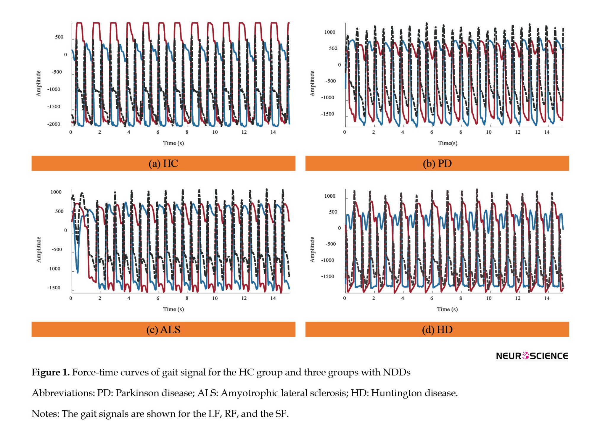
Our study utilized gait in the NDD database (GaitNDD), developed by Hausdorff et al. (2000) and available on the Physionet website (GaitNDD Data Repository, 2019). There are gait recordings of 20 patients with HD, 13 with ALS, 15 with PD, and 16 HC subjects. The recordings are produced using force-sensitive resistors placed under the foot during a 77-m walking trial. Each of the 64 records contains 5-minute gait signals sampled at 300 Hz with a 12-bit analog-to-digital converter. Figure 1 depicts the gait signal of the proposed dataset and their altered gait rhythm.
Study methods
This study proposes two TF gait analysis methods for diagnosing three types of NDDs. Three distinct types of gait signals were employed as input in our study: The left foot (LF), the right foot (RF), and the summation of both feet (SF). In gait analysis, it is imperative to account for leg coordination. To this end, a singular movement signal from one foot would not suffice. Therefore, to accurately capture the gait dynamics, we opted to total up the force applied by each foot.
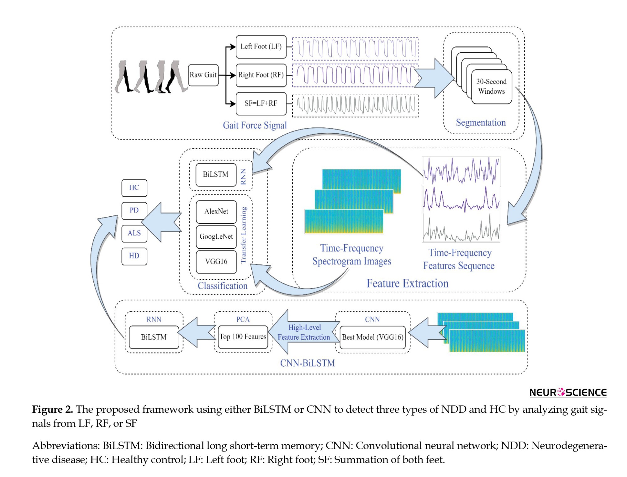
At the outset, these three distinct types of gait signals were uniformly segmented into 30-s windows. Two TF moments were extracted from each segment to be utilized as input for the BiLSTM model. Subsequently, these TF features were translated into 2D spectrogram images for implementation in pre-trained CNNs. The proposed framework is given in Figure 2.
Segmentation
The segmentation function used in this analysis disregards signals with a duration of less than 30 s. Additionally, signals that exceed 30 s are divided into 30-s windows, with any remaining portion of the signal being disregarded. For example, a signal lasting 280 s would be divided into 9 signals of 30 s each, with the remaining 20 s being ignored. This segmentation may not only shorten the time of feature extraction and training of the network, but it may also contribute to making our method more suitable for real-time applications. It should be noted that certain gait patterns may occur during shorter periods of walking that may not be apparent during extended periods. Furthermore, it is more convenient for the patient to record a shorter signal during a real-time clinical diagnosis.
Time-frequency features
A great deal of information in the vGRF signals can be used to analyze and characterize gait. For clinical purposes, the vGRF signal can determine the importance of its spatiotemporal characteristics, such as swing phase, stance phase, and stride time. A TF transform has been applied to gait signals to extract two transient TF features. Therefore, we decided to extract instantaneous frequency (IF) and spectral entropy (SE) as features. IF provides insights into the time-varying frequency components of signals, while SE quantifies the complexity and distribution of energy across different frequency bands.
IF
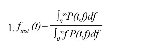
A non-stationary signal’s IF is a time-varying parameter that measures the signal’s average frequencies as it evolves over time (t) (Boashash, 1992a; Boashash, 1992b). In this case, the IF is calculated as the first conditional spectral moment of the TF distribution of x. First, it computes the spectrogram power spectrum P (t, f) of the input signal using the short-time Fourier transform (STFT) and uses the spectrum as a TF distribution. Secondly, it estimates the IF using Equation 1.
SE
A signal’s SE is a measure of its spectral power distribution. The SE value is a measure of the complexity or randomness of the signal across different frequency bands. In the frequency domain, the SE calculates the Shannon entropy of the signal’s normalized power distribution. A high SE value indicates a more complex or unpredictable signal. SE is calculated using the Equation 2:
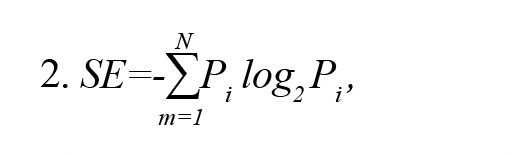
where Pi is the power spectral density (PSD) at a given frequency band. To calculate Pi, the signal x(n) is first divided into overlapping segments of a certain length. Then, a fast Fourier transform is applied to each segment to obtain the PSD estimate: S (m)=|X(m)|2, where X(m) is the discrete Fourier transform of x(n). Finally, the PSD estimates from all segments are averaged to obtain the final PSD estimate for the signal. Once the PSD estimate is obtained, the Pi values can be calculated by dividing the PSD estimate into non-overlapping frequency bands and summing the PSD values within each band. The Pi values are then normalized by dividing by the total power in the signal.
Spectrogram of vGRF
A spectrogram image approach was considered for the 2D representation of the aforementioned features. To compute the time-dependent spectrum of a non-stationary signal, this function separates the signal into overlapping segments, windows each segment using a Kaiser window, calculates STFT, and concatenates the transform matrices. The Equation for STFT can be written as follows (Equation 3):
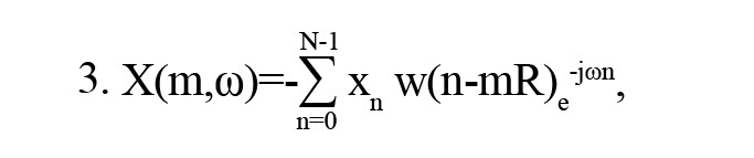
where X(m,ω) represents the complex spectrum at time frame m and frequency ω. xn is the input signal in the time domain. w(n) is a window function applied to the signal to reduce spectral leakage. N is the window size. R is the hop size, which determines the amount of overlap between consecutive windows. e-jωn represents the complex exponential used to decompose the signal into its frequency components. The resulting spectrum is then plotted over time to create a visual representation of the vGRF signal, with the intensity of the color indicating the power or amplitude of the corresponding frequency at each point in time.
BiLSTM architecture
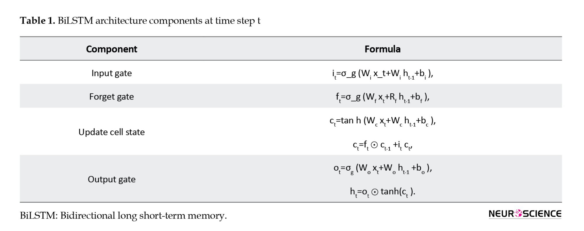
BiLSTM (Schuster & Paliwal, 1997) is a powerful DL architecture and recurrent NN (RNN) type designed to handle long-term dependencies in sequential data. BiLSTMs are particularly effective when the context on both sides of a particular point in a sequence is important in making a prediction. The main idea behind a BiLSTM is to process the input sequence forward and backward through two separate LSTMs and then concatenate their outputs at each time step to obtain the final output. The description of BiLSTM can be broken down into the following steps and equations shown in Table 1:
● The input gate controls how much new information is added to the cell state at the current time step.
● Forget gate controls how much information from the previous cell state should be retained.
● Update cell state: It combines the new input information and the previous cell state information to form a new cell state.
● The output gate controls how much of the current cell state is output as the hidden state.
● Backward LSTM is when the input sequence is processed in reverse through a separate LSTM, and the outputs are concatenated with the forward LSTM outputs at each step.
● The final output of BiLSTM is obtained by concatenating the forward and backward LSTM outputs at each time step.
In Table 1, it, ft, and ot are the input, forget, and output gates, respectively, gt is the candidate memory cell value, ct is the current memory cell value, ht is the current hidden state, ht-1 is the hidden state of the previous time step, xt is the input at time step t, W and b are the weights and biases, respectively. Also, σ and represent the sigmoid and element-wise multiplication operations, respectively, and tanh is the hyperbolic tangent activation function.
BiLSTM allows the model to capture both past and future dependencies in a sequence, which can improve its performance on many sequence labeling tasks. The settings of the BiLSTM network play a crucial role in determining the model's performance during training. The training environment involves a process of trial and error to determine the optimal parameters for our model. To accomplish our objectives, we determined that the adaptive moment estimation optimizer was an effective solver. Moreover, we set a hidden unit number in the BiLSTM layer to 100, an initial learning rate of 0.01 with a maximum epoch of 80, and a mini-batch size of 100. The remaining hyperparameters were set to their default values as defined by MATLAB software, version 2022b.
Transfer learning CNNs
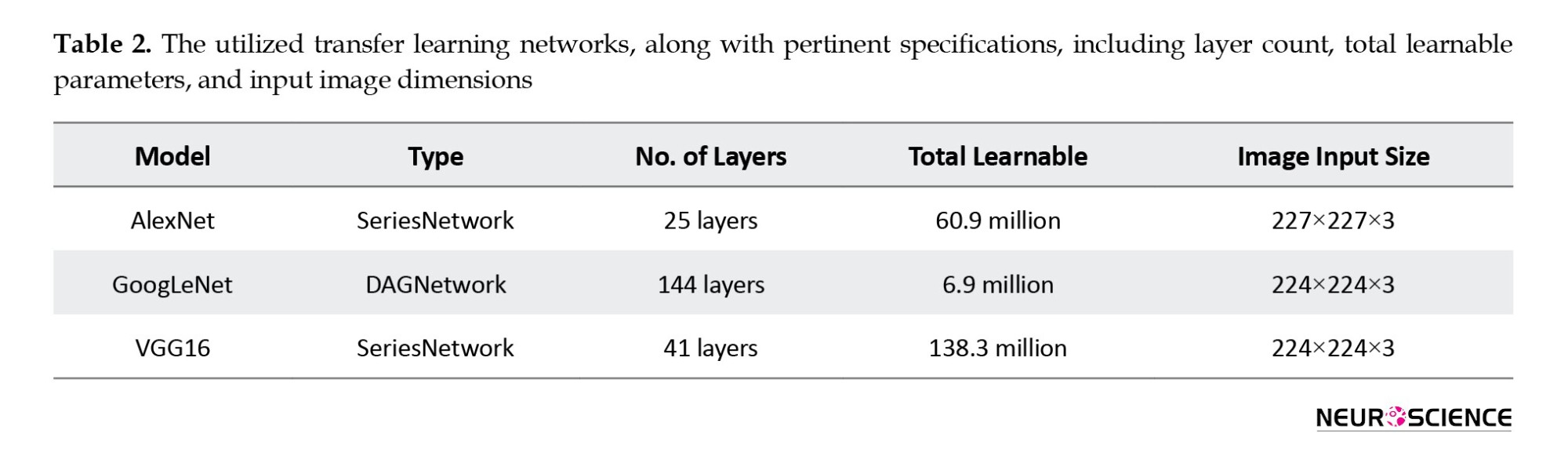
Developing a deep CNN from scratch is computationally intensive and requires substantial training data. Insufficient training data is available in several applications, and generating new realistic training instances is impossible. In these situations, employing CNNs trained on huge data sets for conceptually comparable tasks is beneficial. The use of current CNNs is known as transfer learning (Abedinzadeh Torghabeh et al., 2023; Asghari & Hosseini, 2022; Tuib et al., 2023). AlexNet (Krizhevsky et al., 2017; Modaresnia et al., 2024), GoogLeNet (Szegedy et al., 2015; Abedinzadeh Torghabeh et al., 2023), and VGG16 (Simonyan & Zisserman, 2014) are deep CNN architectures designed for image classification tasks, achieving state-of-the-art performance on the ImageNet dataset, which contains over one million images across 1,000 categories. Table 2 summarizes the types of utilized networks: Directed acyclic graph (DAG) or series networks. It also provides information about the number of layers, the total learnable parameters, and the size of input images.
Three methods can be utilized to transfer learning of these models: Fine-tuning, feature extraction, and domain adaptation. The fine-tuning method involved transferring the weights from the pre-trained model and freezing the selected model’s pre-trained layers. The input of the selected models consists of 30-s TF spectrogram images derived from the vGRF signal, which should be resized to align with the model’s input size. The selected models’ last layers should also be modified to accommodate this study’s four classes under investigation.
These models were trained using stochastic gradient descent with momentum as the solver and weight decay with a momentum value of 0.9. The mini-batch size determines the number of samples used in each iteration to update the weights, which was set to 32, and the maximum number of epochs was set to 10 to prevent overfitting, and the data were shuffled in every epoch to avoid any bias in the training process. The learning rate determines the step size taken during optimization, which is initialized to 3e-4. These settings have been carefully selected to optimize the model’s performance for the given task. The default values for the remaining hyperparameters were used as specified by MATLAB.
3. Results
The present study uses a deep, intelligent, lightweight model to examine the gait signals of individuals with NDD and accurately classify each group solely based on their non-invasive force walking information.
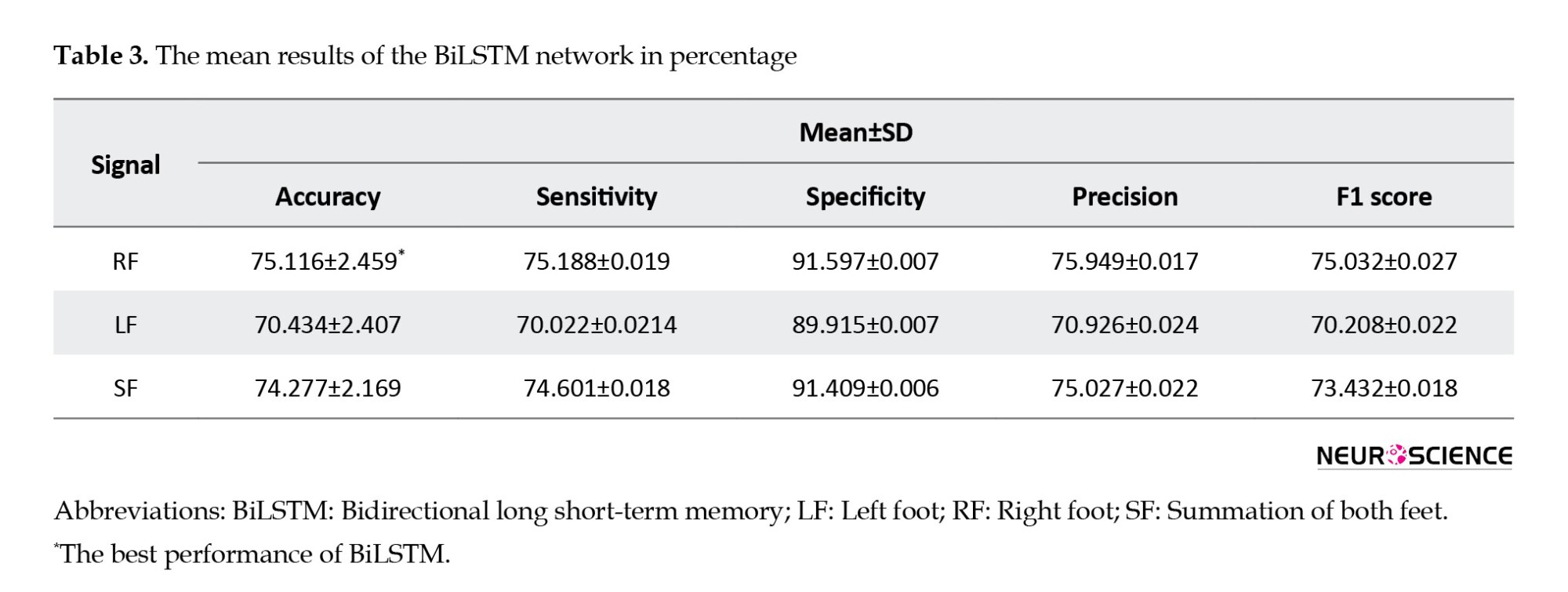
Tables 3 and 4 present the outcomes of the BiLSTM and CNN models in classifying 3 distinct vGRFs, respectively. This information is presented as mean percentages and SD during a 5-fold CV. CNN showed better results, over 99.21% accuracy for all types of RF, LF, and SF signals, compared to BiLSTM, which achieved 70.43% up to 75.11% accuracy.
BiLSTM
Table 3 presents the performance results of the BiLSTM model. The accuracies achieved were 75.11% for RF, 70.43% for LF, and 74.27% for SF. The model exhibited a notable average specificity of 91.597% in effectively discriminating the RF signals associated with distinct groups. In the classification of SF, the model achieved the same specificity percentage, further highlighting its ability to distinguish each group within the dataset effectively.
CNN
The TF spectrogram representation of each vGRF signal for the HC group and different NDDs is shown in Figure 3.
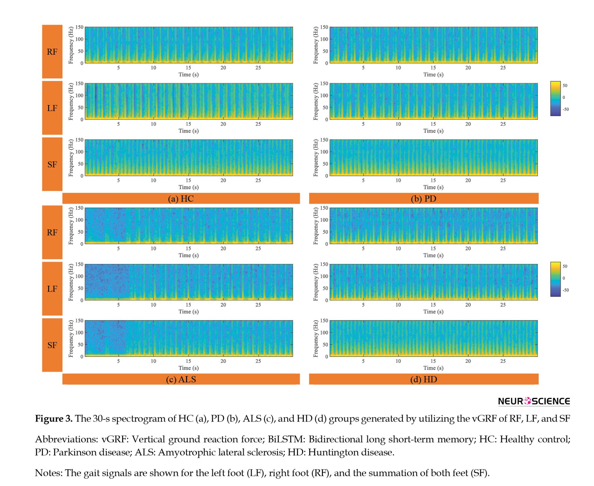
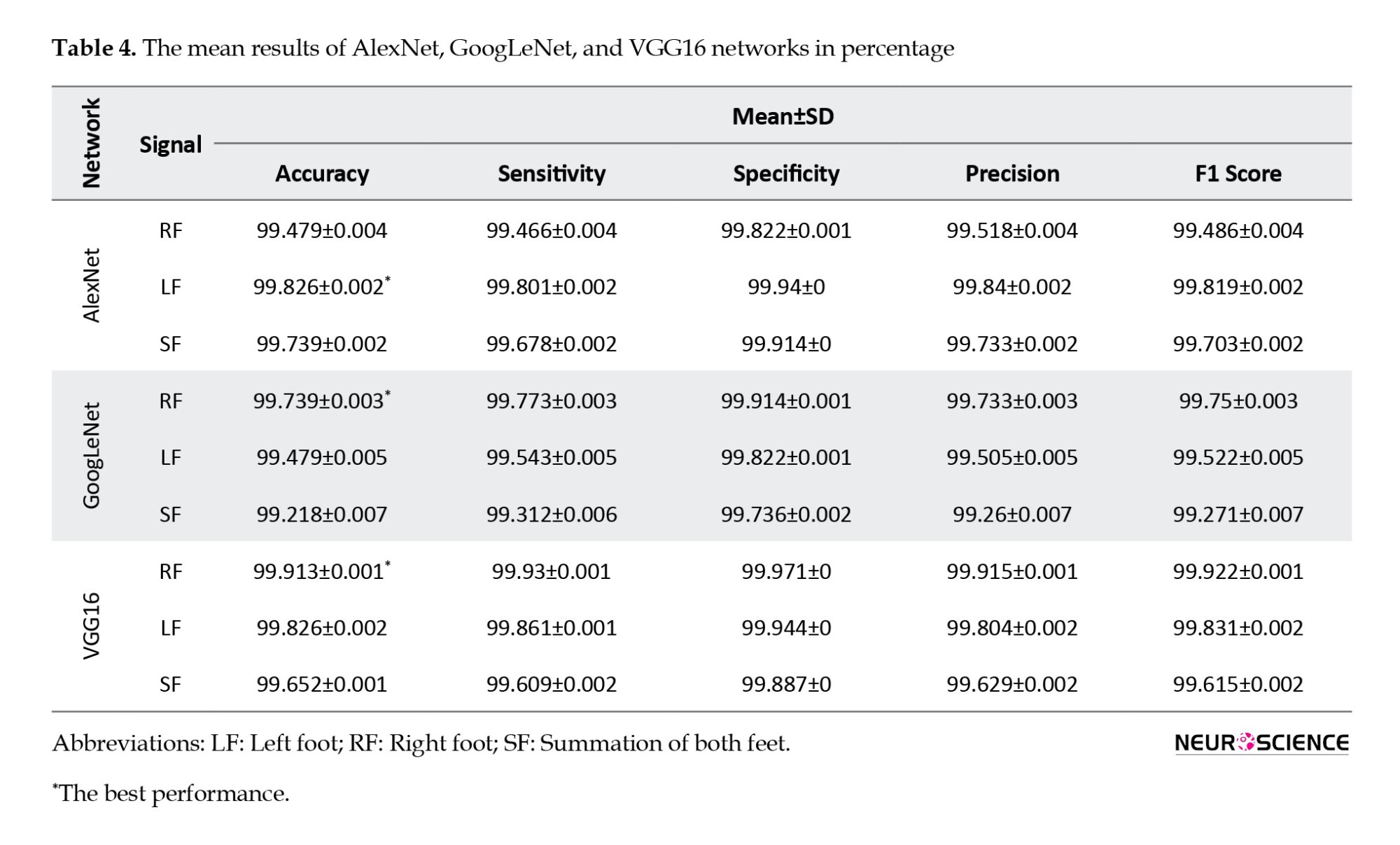
Table 4 shows that among the 3 models, i.e. VGG16, AlexNet, and GoogLeNet, VGG16 achieved the highest accuracy for all 3 TF images of the RF, LF, and SF, with accuracies of 99.91%, 99.82%, and 99.65%, respectively. While the accuracy percentages suggest that VGG16 outperforms the other models, it is important to note that these conclusions are based on reported metrics alone. The AlexNet and GoogLeNet models also performed well, with accuracies ranging from 99.21% to 99.73% for all 3 signals. All models specificity, sensitivity, precision, and F1 scores were consistently high, exceeding 99%, indicating strong overall performance in classifying vGRFs from spectrogram images. However, we acknowledge the need for statistical validation in future work to avoid overstating the results.
Given that both CNNs and BiLSTM utilize features derived from the same TF transform method, these results suggest that CNNs perform better than BiLSTM for analyzing vGRF signals when employing 2D versus 1D feature representations. It is important to note that this study did not include hyperparameter optimization, which may have impacted its performance.
In this study, we aim to explore the patterns of gait signals, specifically the RF, LF, and SF, to discern which signal provides more informative insights into the classification of various NDDs. RF signal had better accuracy in GoogLeNet, VGG16, and BiLSTM. Only in AlexNet, LF showed a better result with 99.82%, which is only 0.35% more accurate than RF signal.
VGG16-BiLSTM
In the RNN approach, utilizing BiLSTM alone did not yield satisfactory outcomes. To address this limitation, we employed a feature enhancement methodology. We used pre-trained CNN with the best performance as a feature extractor and subsequently fed the extracted features to BiLSTM. In the previous experiment utilizing a CNN approach, the VGG16 network was provided with images of the LF, RF, and SF, and it demonstrated superior performance in extracting high-level features compared to the other two CNNs. The resulting CNN-BiLSTM network remarkably improved in accurately distinguishing between 4 classes of NDDs and the HC group.
The rationale behind the approach adopted in this study is based on the fact that CNNs such as VGG16 consist of multiple layers, with each layer learning increasingly abstract representations of the input data. Consequently, deeper layers in the network tend to contain higher-level features constructed using the lower-level features of earlier layers. To leverage this characteristic and extract the most important features, 4096 features were initially extracted from the 36th layer of the VGG16, which is a fully connected layer.
To further enhance the data’s comprehensibility and reduce the feature space’s dimensionality while retaining as much information as possible, PCA was applied to reduce the initial feature dimension from 4096 down to 100 features. The first 100 principal component coefficients were retained, as they were deemed to capture the most relevant information. Finally, the reduced set of features was obtained by projecting the original feature matrix onto the reduced feature space defined by the selected principal component coefficients. This final step resulted in a feature matrix with the same number of rows as the original feature matrix but with only 100 columns, effectively reducing the dimensionality of the feature space and retaining the most essential features. Then, the obtained features were normalized by subtracting the mean of each sample from it and then dividing it by SD.
The network was configured with 100 hidden units, and the training process was set to run for a maximum of 80 epochs. A mini-batch size of 100 was utilized during training, while the initial learning rate was set to 0.01. Additionally, a gradient threshold of 1 was imposed during training to prevent exploding gradients. These network settings were selected based on prior research and were deemed appropriate for the current study’s objectives.
Comparing Tables 3 and 5, we found that the VGG16-BiLSTM architecture demonstrates efficacy in accurately classifying NDDs and HC individuals, with a notable 24% improvement in performance over the basic BiLSTM model. Specifically, as illustrated in Table 5, the model achieved an average accuracy of 99.21% in classifying SF gait signals. Furthermore, the specificity, sensitivity, precision, and F1 were increased by more than 20%. This noteworthy enhancement serves as compelling evidence for the effectiveness of this approach in enhancing the classification results. The method’s ability to significantly elevate these performance metrics highlights its potential for optimizing the accuracy and reliability of the classification process, making it a valuable contribution to the field.
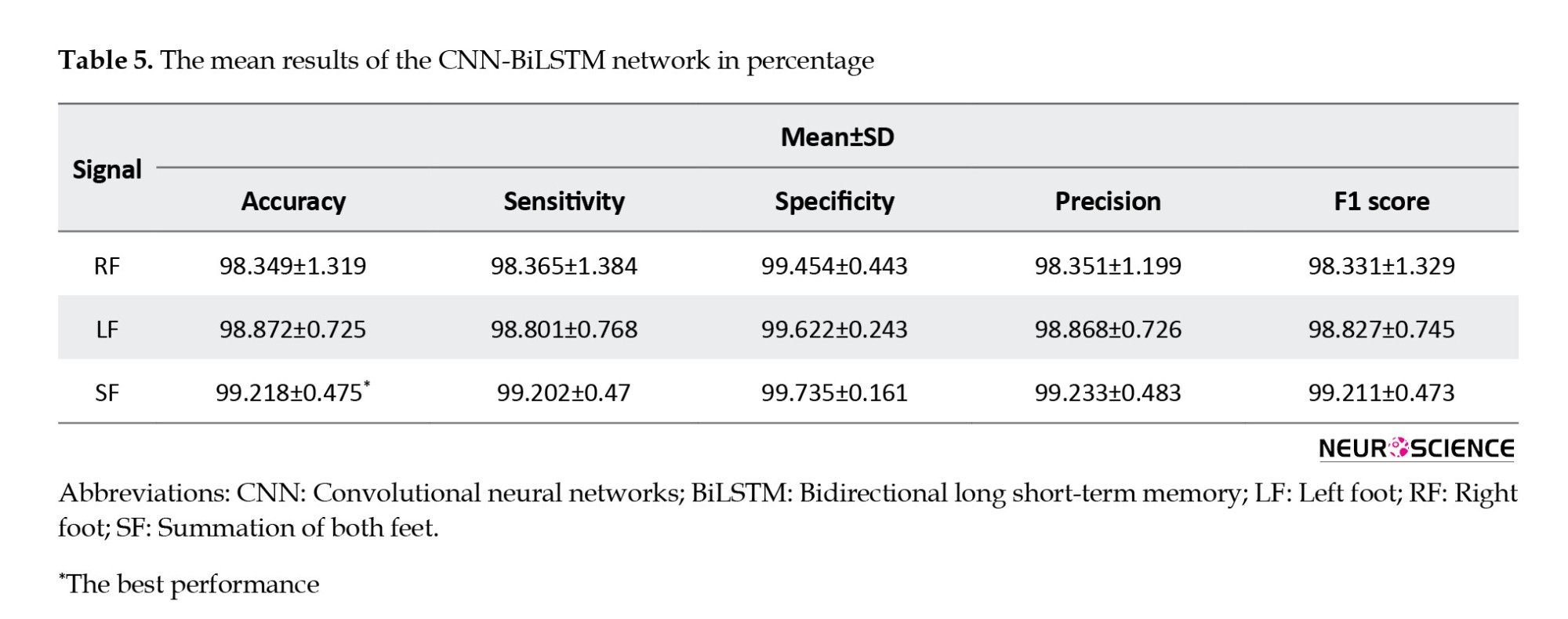
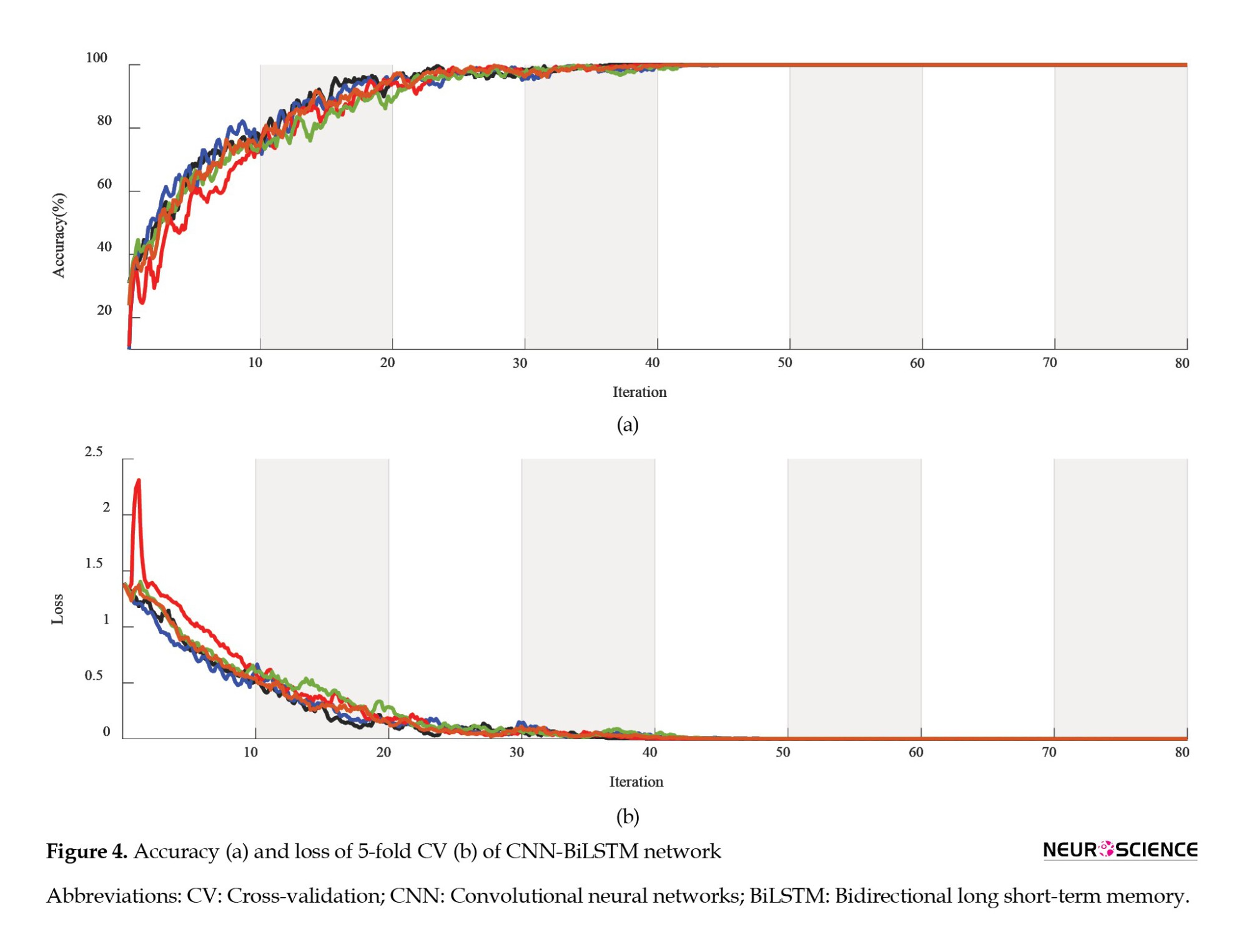
The high level of accuracy observed in the SF gait pattern suggests that this particular pattern may hold potential benefits for computer-aided diagnosis in gait-related contexts. It may provide informative insights beyond those gleaned from individual LF or RF patterns analysis alone. Figure 4 depicts the accuracy and loss curve of the VGG16-BiLSTM network architecture, which underwent a five-fold CV process, and illustrates how the model’s performance gradually converges through 80 epochs. Each graph color represents a separate fold used during the validation process.
4. Discussion
NDDs are a group of disorders characterized by the progressive loss of neurons in the brain or spinal cord, leading to functional impairment and disability. The early detection and diagnosis of these diseases are crucial for effective management and treatment. The analysis of gait signals can provide valuable insights into the motor function of individuals with NDD and aid in the early diagnosis and treatment of related conditions. Using a deep, lightweight method can facilitate the accurate and time-saving classification of different NDD groups, improving the overall well-being of affected individuals.
The primary aim of this investigation is to propose a methodology that is strong, economical, and non-intrusive, which has the potential to strike a better balance between cost and computational complexity while achieving high detection accuracy. Given that previous studies (Ghoreshi Beyrami & Ghaderyan, 2020; Pham, 2018; Setiawan and Lin, 2021a) efficient treatment planning, and monitoring of disease progression. The detection algorithm comprises a preprocessing process, a feature transformation process, and a classification process. In the preprocessing process, the five-minute vGRF signal was divided into 10, 30, and 60 s successive time windows. In the feature transformation process, the time–domain vGRF signal was modified into a time–frequency spectrogram using a CWT achieved perfect average accuracy in binary classification, we decided to exclude the binary classification task between the disease groups and HC subjects. Instead, our focus shifted to multi-class classification.
The proposed deep TF study provides valuable insights into the health status of the cohort, as it allows for the identification of potential abnormalities or anomalies in the vGRF. This methodology presents a comprehensive and impartial evaluation of the TF features in gait signals by utilizing and comparing feature sequences, IF and SE, as inputs for BiLSTM and their corresponding spectrogram images for CNNs. Earlier investigations have underscored the significance of frequency (Joshi et al., 2017) and high-level spectrogram features (Setiawan and Lin, 2021a, Setiawan & Lin, 2021b) in NDD classification. Building upon these findings, we employed a comprehensive approach encompassing frequency-based and high-level spectrogram features. The objective was to discern the most effective feature representation in 1D or 2D form. Our proposed study revealed the prevalence of auto-extracted features, indicating their superiority over other data-driven features in NDD classification. This comparative analysis allowed us to uncover valuable insights into the optimal choice of features for improved accuracy and performance to facilitate the diagnosis and classification of NDD.
The findings of this investigation demonstrate that employing spectrogram images to feed the CNNs, which convert time-domain signals into frequency-domain representations, provides a more comprehensive view of the vGRF signal than traditional 1D time-domain representations. Analyzing these spectrogram images using DL techniques makes it possible to extract the temporal and spectral high-level features that capture the important characteristics to understand the underlying signals better. High-level features extracted from CNNs provide valuable information regarding the levels of abstraction present in an image. The earlier layers of the network detect lower-level features, such as edges and corners, while the later layers detect higher-level features, such as shapes and objects. Moreover, visualizing in-depth features facilitates understanding how the model makes its predictions.
The combination of CNNs and spectrogram images has proven to be a powerful tool for feature extraction in vGRF signal processing tasks. The ability of CNNs to automatically learn high-level features from raw data, combined with the rich information provided by spectrograms, has led to significant improvements in accuracy and robustness compared to traditional hand-crafted feature extraction methods. Moreover, The high level of accuracy observed in the SF vGRF suggests that this particular gait pattern may hold potential benefits for computer-aided diagnosis in gait-related contexts. It may provide informative insights beyond those gleaned from individual LF or RF patterns analysis alone.
Table 6 presents a comparative analysis of the latest research studies in the field employing diverse ML techniques and DL networks, including CNN or RNN architectures. Notably, the Table highlights a superior performance of the proposed method compared to prior multi-class NDD detection methods utilizing the identical dataset. The VGG16-BiLSTM approach, with 99.21% accuracy, also outperforms other studies that use the DL approach for the four-class classification of NDDs.
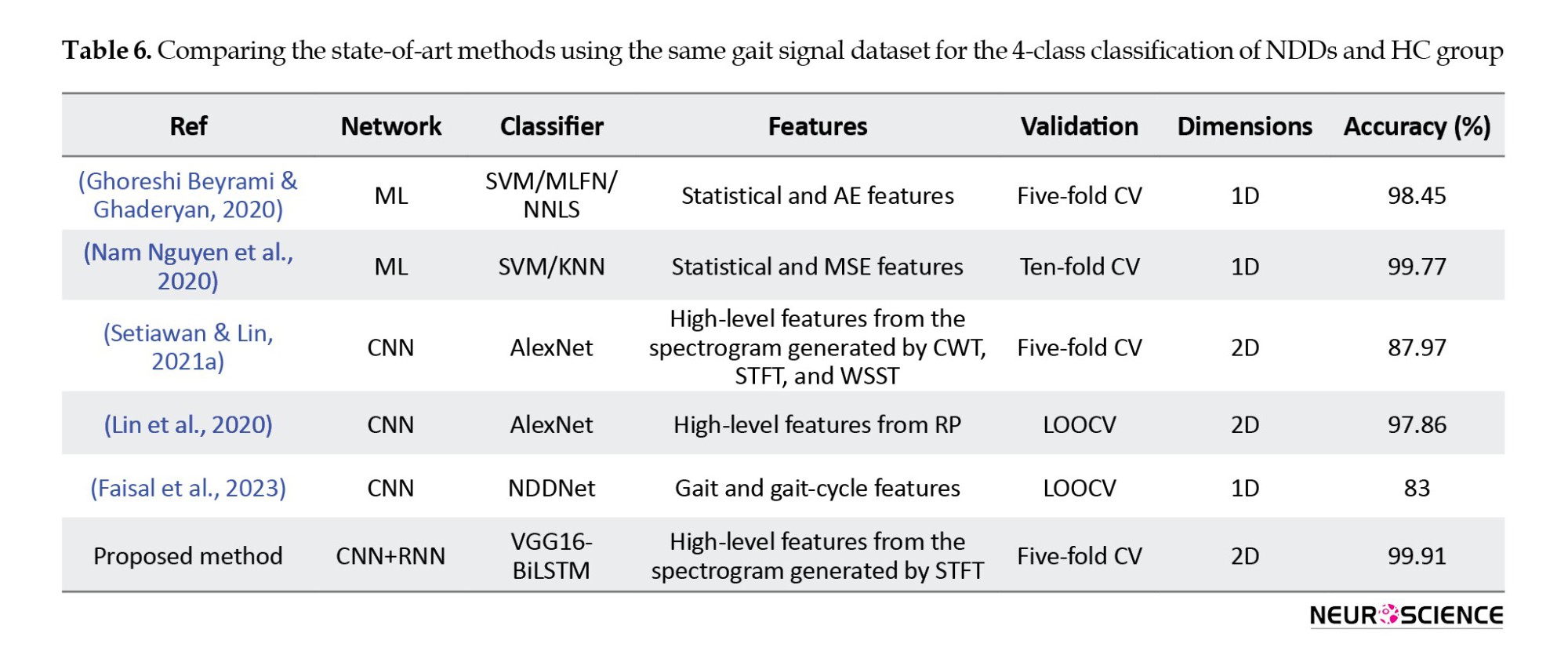
The CNN and CNN-BiLSTM models employed in the present investigation have been determined to be reliable diagnostic tools for NDD, exhibiting minimal SD throughout the 5-fold CV.
5. Conclusion
This study demonstrates the effectiveness of BiLSTM and CNNs in accurately detecting NDD from vGRF signals obtained through wearable force sensors. Two experimental trials were conducted; two informative TF features were extracted from the vGRF of patients’ right, left, and combined feet during a walking task, which were then used to feed a BiLSTM network. In the second trial, equivalent spectrogram images of the vGRF signal were constructed as input for CNNs. The findings demonstrate that utilizing transfer learning with VGG16 yielded superior outcomes in the automatic identification of NDDs, with accuracy, sensitivity, and specificity rates of 99.91%, 99.93%, and 99.97%, respectively. The significant promotion in the BiLSTM network performance was also achieved by feeding high-level features extracted from VGG16 instead of hand-crafted features. Overall, the CNN high-level features extracted from the spectrogram derived from the vGRF signal can provide valuable insights into the underlying NDD group and help researchers better understand the mechanisms of vGRF in different NDDs.
Ethical Considerations
Compliance with ethical guidelines
According to the data description, all ethical principles were strictly followed during the data-gathering procedure. Participants were fully informed about the purpose of the research, the implementation stages, and the procedures involved. They were assured of the confidentiality of their information and had the freedom to withdraw from the study at any time without any consequences. Additionally, they were offered access to the research findings upon request. Written informed consent was obtained from all participants, and the principles of the Helsinki Declaration were thoroughly observed.
Funding
This research did not receive any grant from funding agencies in the public, commercial, or non-profit sectors.
Authors' contributions
Conceptualization, methodology, software, data curation, and writing the original draft; Farhad Abedinzadeh Torghabeh; Visualization: Yeganeh Modaresnia, and Farhad Abedinzadeh Torghabeh; Supervision, investigation, and validation: Seyyed Abed Hosseini; Review and editing: Yeganeh Modaresnia, Seyyed Abed Hosseini;
Conflict of interest
The authors declared no conflict of interest.
Acknowledgments
The authors want to express their sincere gratitude to Jeffrey M. Hausdorff for providing the gait in the Neurodegenerative Disease Database, which was made publicly available. The availability of this valuable dataset has dramatically facilitated our research and contributed to the findings presented in this study.
References
Neurodegeneration is the gradual loss of structure and function of neurons in a disease known as a neurodegenerative disease (NDD). Ultimately, such neuronal damage may result in the death of the cells. NDDs include Parkinson disease (PD), amyotrophic lateral sclerosis (ALS), multiple sclerosis, Alzheimer disease (AD), Huntington disease (HD), multiple system atrophy, and prion diseases (Stephenson et al., 2018). PD, ALS, and HD are a group of NDDs characterized by motor impairment due to the gradual decline of motor neurons in the presence of protein aggregates at different brain regions (Ghaderyan & Ghoreshi Beyrami, 2020; Zeng & Wang, 2015). Clinically, these NDDs manifest as hyperkinetic movements, bradykinesia, tremors, rigidity, and progressive muscle atrophy (Ghoreshi Beyrami & Ghaderyan, 2020). Additionally, these patients are more likely to fall or sustain physical injuries due to their abnormal movements (Allen et al., 2013; Vuong et al., 2018) 60.5% (range 35 to 90%.
After AD, PD is the second most frequent NDD. It is estimated that the age-sex-adjusted incidence of PD in North America varied from 108 to 212 per 100000 people aged 65 and older and from 47 to 77 per 100000 people aged 45 and older. The prevalence of PD rose with age and was more significant in men (Willis et al., 2022). The following motor symptoms often characterize PD: Trembling, bradykinesia (slowed movement), rest tremor (rhythmic shaking), rigidity, reduced postural reflexes, and impaired balance (Abedinzadeh Torghabeh et al., 2023; Váradi, 2020). ALS is the third most widespread NDD and the most prevalent motor neuron disease, with an estimated incidence of 1.9 per 100000 persons annually. In Europe and the United States, the annual incidence of ALS is approximately 2.3 per 1000 persons (Xu et al., 2020). ALS is characterized by increasing muscular weakness, muscle atrophy, fasciculations, muscle spasms, slow movement, and muscle stiffness. The beginning of muscular weakness in ALS is often localized and extends to neighboring body parts (Masrori & Van Damme, 2020). HD is a hereditary neurological disorder characterized by involuntary jerky movements and shaky gait with cognitive and behavioral impairment. These involuntary movements begin in the distal extremities and are of lesser severity, although they may also affect the facial muscles. The signs gradually spread to the proximal and axial muscles and become more pronounced. Typically, motor symptoms are progressive (Roos, 2010) behavioral and psychiatric disturbances and dementia. Prevalence in the Caucasian population is estimated at 1/10,000-1/20,000. Mean age at onset of symptoms is 30-50 years. In some cases symptoms start before the age of 20 years with behavior disturbances and learning difficulties at school (Nopoulos, 2021).
The clinical diagnosis of NDDs is widely considered one of the most crucial areas of biomedical engineering research because these disorders affect an increasing number of people worldwide physically, psychologically, and financially (Erkkinen et al., 2018). The importance of a correct diagnosis will increase when disease-modifying therapies become available. There is potential for widespread clinical use of diagnostic biomarkers that are easy to access, cost-effective, and accurate (Hansson, 2021). A misdiagnosis may result in inadequate treatment, unnecessary care-seeking, and cost-prohibitive investigations due to diagnostic uncertainty.
Several techniques are often employed to diagnose such NDDs, including functional neuroimaging, genetic blood tests, spinal cord imaging, and nerve-muscle biopsy. These techniques allow us to examine brain structure, function, and pathology and investigate neurodegenerative mechanisms in vivo. As a result of movement impairment in NDDs, it is reasonable to conclude that NDDs also affect foot force, resulting in the use of gait modality. The gait data have been used to analyze movement and balance abnormalities in healthy controls (HCs) and subjects with various diseases. In particular, measuring the biomechanical properties of gait during walking can provide valuable insights into the movement pattern of NDDs and has great promise for developing non-invasive automated NDD classification techniques.
Wearable gait sensors have significantly reduced the need for costly laboratory equipment and specialized supervision. Force sensors have gained widespread acceptance among the various gait sensors due to their exceptional accuracy in mapping joint movements and muscle activities (Abedinzadeh Torghabeh et al., 2023). These sensors are highly popular in gait analysis research owing to their non-invasive nature, compact size, and affordability (Roelker et al., 2019). As a result, they have become one of the most commonly utilized tools in gait analysis studies (Abedinzadeh Torghabeh et al., 2023). Several gait parameters, such as stride length, stride time, step width, and gait velocity, alter in patients with NDDs compared to HC. These alterations are often subtle and may not be visible to the naked eye but can be detected using advanced gait signal analysis techniques such as machine learning (ML) algorithms.
Recently, gait analysis has emerged as a promising non-invasive tool for detecting NDDs, providing valuable insights into the underlying motor impairments associated with these diseases. In this literature review, we will explore the current state of research on gait signal analysis for detecting NDDs, which all focus on PD, ALS, and HD and their matched HC.
Pham (2018) discussed a gait analysis approach by transforming feature sequences into 2-dimensional (2D) texture images using the fuzzy recurrence plot (FRP) algorithm. The gray-level co-occurrence matrix (GLCM) is then used to extract 19 texture features from FRP images of HC and 3 groups of NDDs. Then, the least square support vector machine (SVM) was used to differentiate HC from PD, ALS, and HD, where an accuracy rate of 100% was achieved. Gupta et al. (2019) proposed a methodology based on statistical and entropic features of the vertical ground reaction force (vGRF) signal, along with autocorrelation and cross-correlation between gait time series. They used a rule-based classifier trained with a decision tree algorithm and performed mutual information analysis to evaluate the effectiveness of different feature sets. Their approach achieved accuracy from 87.5% to 96.2% for binary classification of different NDDs and HCs.
Ghoreshi Beyrami & Ghaderyan, (2020) presented a methodology for diagnosing three types of NDDs based on Mean±SD, skewness, kurtosis, and approximate entropy (AE) features of vGRF signals and sparse non-negative least squares (NNLS) coding classification technique, where their model achieved 100%, 99.78%, and 99.60% for ALS, PD, and HD detection tasks, respectively. Also, they could classify NDD and HC, achieving an accuracy of 98.45%. Nam Nguyen et al. (2020) used the Mean±SD, and multiscale sample entropy (MSE) values for feature extraction and utilized SVM and K-nearest neighbor (KNN) as classifiers. The investigation employed different windows for the segmentation data imbalancement method. They achieved more than 99% accuracy for various binary classifications and a 99.77% accuracy for four-class differentiating between HC and various NDDs.
Prabhu et al. (2020) used recurrence quantification analysis to quantify gait parameters using SVM and probabilistic neural network (NN). Thirteen HC subjects and 13 NDD patients were classified using these models with the Hill-climbing feature selection technique. The two-class accuracy ranged from 96% to 100%. Setiawan and Lin (2021a) efficient treatment planning, and monitoring of disease progression. The detection algorithm comprises a preprocessing process, a feature transformation process, and a classification process. In the preprocessing process, the five-minute vGRF signal was divided into 10, 30, and 60 s successive time windows. In the feature transformation process, the time–domain vGRF signal was modified into a time–frequency spectrogram using a CWT presented an approach for identifying NDDs using a time-frequency (TF) spectrogram and deep learning (DL) NN features. They focused on the effectiveness of feature transformations from a 1-dimensional (1D) vGRF signal into a 2D TF spectrogram, combined with principal component analysis (PCA) and convolutional NN (CNN) as a feature extractor for the classification of NDD patients, at which their model attained an accuracy of 87.97% through 5-fold cross-validation (CV) and 97.42% through leave-one-out CV (LOOCV). In another study, Setiawan and Lin (2021b) which are subjective and can be inaccurate. These techniques are not very reliable, particularly in the early stages of the disease. A novel detection and severity classification algorithm using deep learning approaches was developed in this research to classify the PD severity level based on vGRF (vGRF used preprocessing, feature transformation, and classification processes, including dividing the vGRF signal into successive time windows, transforming it into a TF spectrogram using continuous wavelet transform (CWT), enhancing features with PCA, and employing CNNs for classification, wherein they achieved an accuracy of 96.52% using ResNet-50 in classifying PD severity levels.
Erdaş et al. (2021) proposed two new models which first detect NDDs by converting GRF to 2D quick-response (QR) code images based on convolutional long short-term memory (ConvLSTM) and then 3-dimensional (3D) tensors extracted with ConvLSTM fed to 3D CNN to classify three NDDs. Their model was accurate by 95.73% in classifying NDDs and HC through the 10-fold CV. Lin et al. (2020) used recurrence plot (RP) image feature extraction to improve the accuracy of NDD diagnosis. The algorithm transformed the vGRF signal into RP images and applied a CNN for classification. In the 2-class classification, the accuracy was from 95.95% to 100%, while in the 4-class, their model was accurate by 97.86% on average through LOOCV.
Faisal et al. (2023) developed an NN architecture, known as NNDNet, to identify 3 distinct types of NDDs. The model integrated vGRF signals and 14 hand-crafted features, achieving an average accuracy of 83% through LOOCV. Amooei et al. (2023) introduced 2 models based on a CNN-long short-term memory (LSTM) network for classifying NDDs using gait signals transformed into spectrogram images. The first model achieved 99.42% accuracy using CNN-LSTM, while the second model, which used wavelet transform as a feature extractor and CNN-LSTM, achieved an accuracy of 95.37% using only approximation sub-bands.
These studies demonstrated that DL algorithms have gained popularity and shown promising results in accurately classifying gait signals for the automated diagnosis of NDDs, highlighting their potential as a valuable tool for medical diagnosis and treatment.
This study attempts to establish a prognostic solution for classifying NDDs utilizing conveniently obtainable data from wearable sensors. In light of this, an intelligent tool can detect NDDs based on gait data. Moreover, given the significant dearth of research focused on multi-class classification, this investigation distinguishes itself from conventional gait analysis methodologies by prioritizing enhancing 4-class classification effectiveness. This approach allowed us to explore the complexity of multi-class classification and gain a deeper understanding of the distinctive patterns and characteristics among the various disease groups. Our proposed method contributes in 4 significant capacities. First, this study offers 2 TF models for accurately and reliably classifying NDD patients from the vGRF signal using bidirectional LSTM (BiLSTM) and CNN. Secondly, this study examines the effectiveness of feature transformations from a 1D vGRF signal to a 2D TF spectrogram. Thirdly, this research presents a highly efficient approach for identifying NDDs, which may be incredibly useful for clinical decision support systems and obtain the most significant classification accuracy for three types of NDDs. Our suggested technique outperformed existing models employed in prior research to predict NDDs. Last, we have enhanced the efficiency of BiLSTM by incorporating the top-performing high-level features of the best CNN model into BiLSTM.
The current study was organized into the following sections. First, section 2 delves into the existing research on automated techniques for diagnosing NDDs. Section 3 presents the materials and methods employed in this study. Subsequently, section 4 presents the experimental findings, and Section 5 argues corresponding discussions. Finally, Section 6 concludes the study.
2. Materials and Methods
The proposed study investigates the potential of pre-trained DL models for transferring their learned useful features trained on extensive datasets for the non-invasive detection of NDDs through gait signal analysis.
Study materials
Our study utilized gait in the NDD database (GaitNDD), developed by Hausdorff et al. (2000) and available on the Physionet website (GaitNDD Data Repository, 2019). There are gait recordings of 20 patients with HD, 13 with ALS, 15 with PD, and 16 HC subjects. The recordings are produced using force-sensitive resistors placed under the foot during a 77-m walking trial. Each of the 64 records contains 5-minute gait signals sampled at 300 Hz with a 12-bit analog-to-digital converter. Figure 1 depicts the gait signal of the proposed dataset and their altered gait rhythm.
Study methods
This study proposes two TF gait analysis methods for diagnosing three types of NDDs. Three distinct types of gait signals were employed as input in our study: The left foot (LF), the right foot (RF), and the summation of both feet (SF). In gait analysis, it is imperative to account for leg coordination. To this end, a singular movement signal from one foot would not suffice. Therefore, to accurately capture the gait dynamics, we opted to total up the force applied by each foot.
At the outset, these three distinct types of gait signals were uniformly segmented into 30-s windows. Two TF moments were extracted from each segment to be utilized as input for the BiLSTM model. Subsequently, these TF features were translated into 2D spectrogram images for implementation in pre-trained CNNs. The proposed framework is given in Figure 2.
Segmentation
The segmentation function used in this analysis disregards signals with a duration of less than 30 s. Additionally, signals that exceed 30 s are divided into 30-s windows, with any remaining portion of the signal being disregarded. For example, a signal lasting 280 s would be divided into 9 signals of 30 s each, with the remaining 20 s being ignored. This segmentation may not only shorten the time of feature extraction and training of the network, but it may also contribute to making our method more suitable for real-time applications. It should be noted that certain gait patterns may occur during shorter periods of walking that may not be apparent during extended periods. Furthermore, it is more convenient for the patient to record a shorter signal during a real-time clinical diagnosis.
Time-frequency features
A great deal of information in the vGRF signals can be used to analyze and characterize gait. For clinical purposes, the vGRF signal can determine the importance of its spatiotemporal characteristics, such as swing phase, stance phase, and stride time. A TF transform has been applied to gait signals to extract two transient TF features. Therefore, we decided to extract instantaneous frequency (IF) and spectral entropy (SE) as features. IF provides insights into the time-varying frequency components of signals, while SE quantifies the complexity and distribution of energy across different frequency bands.
IF
A non-stationary signal’s IF is a time-varying parameter that measures the signal’s average frequencies as it evolves over time (t) (Boashash, 1992a; Boashash, 1992b). In this case, the IF is calculated as the first conditional spectral moment of the TF distribution of x. First, it computes the spectrogram power spectrum P (t, f) of the input signal using the short-time Fourier transform (STFT) and uses the spectrum as a TF distribution. Secondly, it estimates the IF using Equation 1.
SE
A signal’s SE is a measure of its spectral power distribution. The SE value is a measure of the complexity or randomness of the signal across different frequency bands. In the frequency domain, the SE calculates the Shannon entropy of the signal’s normalized power distribution. A high SE value indicates a more complex or unpredictable signal. SE is calculated using the Equation 2:
where Pi is the power spectral density (PSD) at a given frequency band. To calculate Pi, the signal x(n) is first divided into overlapping segments of a certain length. Then, a fast Fourier transform is applied to each segment to obtain the PSD estimate: S (m)=|X(m)|2, where X(m) is the discrete Fourier transform of x(n). Finally, the PSD estimates from all segments are averaged to obtain the final PSD estimate for the signal. Once the PSD estimate is obtained, the Pi values can be calculated by dividing the PSD estimate into non-overlapping frequency bands and summing the PSD values within each band. The Pi values are then normalized by dividing by the total power in the signal.
Spectrogram of vGRF
A spectrogram image approach was considered for the 2D representation of the aforementioned features. To compute the time-dependent spectrum of a non-stationary signal, this function separates the signal into overlapping segments, windows each segment using a Kaiser window, calculates STFT, and concatenates the transform matrices. The Equation for STFT can be written as follows (Equation 3):
where X(m,ω) represents the complex spectrum at time frame m and frequency ω. xn is the input signal in the time domain. w(n) is a window function applied to the signal to reduce spectral leakage. N is the window size. R is the hop size, which determines the amount of overlap between consecutive windows. e-jωn represents the complex exponential used to decompose the signal into its frequency components. The resulting spectrum is then plotted over time to create a visual representation of the vGRF signal, with the intensity of the color indicating the power or amplitude of the corresponding frequency at each point in time.
BiLSTM architecture
BiLSTM (Schuster & Paliwal, 1997) is a powerful DL architecture and recurrent NN (RNN) type designed to handle long-term dependencies in sequential data. BiLSTMs are particularly effective when the context on both sides of a particular point in a sequence is important in making a prediction. The main idea behind a BiLSTM is to process the input sequence forward and backward through two separate LSTMs and then concatenate their outputs at each time step to obtain the final output. The description of BiLSTM can be broken down into the following steps and equations shown in Table 1:
● The input gate controls how much new information is added to the cell state at the current time step.
● Forget gate controls how much information from the previous cell state should be retained.
● Update cell state: It combines the new input information and the previous cell state information to form a new cell state.
● The output gate controls how much of the current cell state is output as the hidden state.
● Backward LSTM is when the input sequence is processed in reverse through a separate LSTM, and the outputs are concatenated with the forward LSTM outputs at each step.
● The final output of BiLSTM is obtained by concatenating the forward and backward LSTM outputs at each time step.
In Table 1, it, ft, and ot are the input, forget, and output gates, respectively, gt is the candidate memory cell value, ct is the current memory cell value, ht is the current hidden state, ht-1 is the hidden state of the previous time step, xt is the input at time step t, W and b are the weights and biases, respectively. Also, σ and represent the sigmoid and element-wise multiplication operations, respectively, and tanh is the hyperbolic tangent activation function.
BiLSTM allows the model to capture both past and future dependencies in a sequence, which can improve its performance on many sequence labeling tasks. The settings of the BiLSTM network play a crucial role in determining the model's performance during training. The training environment involves a process of trial and error to determine the optimal parameters for our model. To accomplish our objectives, we determined that the adaptive moment estimation optimizer was an effective solver. Moreover, we set a hidden unit number in the BiLSTM layer to 100, an initial learning rate of 0.01 with a maximum epoch of 80, and a mini-batch size of 100. The remaining hyperparameters were set to their default values as defined by MATLAB software, version 2022b.
Transfer learning CNNs
Developing a deep CNN from scratch is computationally intensive and requires substantial training data. Insufficient training data is available in several applications, and generating new realistic training instances is impossible. In these situations, employing CNNs trained on huge data sets for conceptually comparable tasks is beneficial. The use of current CNNs is known as transfer learning (Abedinzadeh Torghabeh et al., 2023; Asghari & Hosseini, 2022; Tuib et al., 2023). AlexNet (Krizhevsky et al., 2017; Modaresnia et al., 2024), GoogLeNet (Szegedy et al., 2015; Abedinzadeh Torghabeh et al., 2023), and VGG16 (Simonyan & Zisserman, 2014) are deep CNN architectures designed for image classification tasks, achieving state-of-the-art performance on the ImageNet dataset, which contains over one million images across 1,000 categories. Table 2 summarizes the types of utilized networks: Directed acyclic graph (DAG) or series networks. It also provides information about the number of layers, the total learnable parameters, and the size of input images.
Three methods can be utilized to transfer learning of these models: Fine-tuning, feature extraction, and domain adaptation. The fine-tuning method involved transferring the weights from the pre-trained model and freezing the selected model’s pre-trained layers. The input of the selected models consists of 30-s TF spectrogram images derived from the vGRF signal, which should be resized to align with the model’s input size. The selected models’ last layers should also be modified to accommodate this study’s four classes under investigation.
These models were trained using stochastic gradient descent with momentum as the solver and weight decay with a momentum value of 0.9. The mini-batch size determines the number of samples used in each iteration to update the weights, which was set to 32, and the maximum number of epochs was set to 10 to prevent overfitting, and the data were shuffled in every epoch to avoid any bias in the training process. The learning rate determines the step size taken during optimization, which is initialized to 3e-4. These settings have been carefully selected to optimize the model’s performance for the given task. The default values for the remaining hyperparameters were used as specified by MATLAB.
3. Results
The present study uses a deep, intelligent, lightweight model to examine the gait signals of individuals with NDD and accurately classify each group solely based on their non-invasive force walking information.
Tables 3 and 4 present the outcomes of the BiLSTM and CNN models in classifying 3 distinct vGRFs, respectively. This information is presented as mean percentages and SD during a 5-fold CV. CNN showed better results, over 99.21% accuracy for all types of RF, LF, and SF signals, compared to BiLSTM, which achieved 70.43% up to 75.11% accuracy.
BiLSTM
Table 3 presents the performance results of the BiLSTM model. The accuracies achieved were 75.11% for RF, 70.43% for LF, and 74.27% for SF. The model exhibited a notable average specificity of 91.597% in effectively discriminating the RF signals associated with distinct groups. In the classification of SF, the model achieved the same specificity percentage, further highlighting its ability to distinguish each group within the dataset effectively.
CNN
The TF spectrogram representation of each vGRF signal for the HC group and different NDDs is shown in Figure 3.
Table 4 shows that among the 3 models, i.e. VGG16, AlexNet, and GoogLeNet, VGG16 achieved the highest accuracy for all 3 TF images of the RF, LF, and SF, with accuracies of 99.91%, 99.82%, and 99.65%, respectively. While the accuracy percentages suggest that VGG16 outperforms the other models, it is important to note that these conclusions are based on reported metrics alone. The AlexNet and GoogLeNet models also performed well, with accuracies ranging from 99.21% to 99.73% for all 3 signals. All models specificity, sensitivity, precision, and F1 scores were consistently high, exceeding 99%, indicating strong overall performance in classifying vGRFs from spectrogram images. However, we acknowledge the need for statistical validation in future work to avoid overstating the results.
Given that both CNNs and BiLSTM utilize features derived from the same TF transform method, these results suggest that CNNs perform better than BiLSTM for analyzing vGRF signals when employing 2D versus 1D feature representations. It is important to note that this study did not include hyperparameter optimization, which may have impacted its performance.
In this study, we aim to explore the patterns of gait signals, specifically the RF, LF, and SF, to discern which signal provides more informative insights into the classification of various NDDs. RF signal had better accuracy in GoogLeNet, VGG16, and BiLSTM. Only in AlexNet, LF showed a better result with 99.82%, which is only 0.35% more accurate than RF signal.
VGG16-BiLSTM
In the RNN approach, utilizing BiLSTM alone did not yield satisfactory outcomes. To address this limitation, we employed a feature enhancement methodology. We used pre-trained CNN with the best performance as a feature extractor and subsequently fed the extracted features to BiLSTM. In the previous experiment utilizing a CNN approach, the VGG16 network was provided with images of the LF, RF, and SF, and it demonstrated superior performance in extracting high-level features compared to the other two CNNs. The resulting CNN-BiLSTM network remarkably improved in accurately distinguishing between 4 classes of NDDs and the HC group.
The rationale behind the approach adopted in this study is based on the fact that CNNs such as VGG16 consist of multiple layers, with each layer learning increasingly abstract representations of the input data. Consequently, deeper layers in the network tend to contain higher-level features constructed using the lower-level features of earlier layers. To leverage this characteristic and extract the most important features, 4096 features were initially extracted from the 36th layer of the VGG16, which is a fully connected layer.
To further enhance the data’s comprehensibility and reduce the feature space’s dimensionality while retaining as much information as possible, PCA was applied to reduce the initial feature dimension from 4096 down to 100 features. The first 100 principal component coefficients were retained, as they were deemed to capture the most relevant information. Finally, the reduced set of features was obtained by projecting the original feature matrix onto the reduced feature space defined by the selected principal component coefficients. This final step resulted in a feature matrix with the same number of rows as the original feature matrix but with only 100 columns, effectively reducing the dimensionality of the feature space and retaining the most essential features. Then, the obtained features were normalized by subtracting the mean of each sample from it and then dividing it by SD.
The network was configured with 100 hidden units, and the training process was set to run for a maximum of 80 epochs. A mini-batch size of 100 was utilized during training, while the initial learning rate was set to 0.01. Additionally, a gradient threshold of 1 was imposed during training to prevent exploding gradients. These network settings were selected based on prior research and were deemed appropriate for the current study’s objectives.
Comparing Tables 3 and 5, we found that the VGG16-BiLSTM architecture demonstrates efficacy in accurately classifying NDDs and HC individuals, with a notable 24% improvement in performance over the basic BiLSTM model. Specifically, as illustrated in Table 5, the model achieved an average accuracy of 99.21% in classifying SF gait signals. Furthermore, the specificity, sensitivity, precision, and F1 were increased by more than 20%. This noteworthy enhancement serves as compelling evidence for the effectiveness of this approach in enhancing the classification results. The method’s ability to significantly elevate these performance metrics highlights its potential for optimizing the accuracy and reliability of the classification process, making it a valuable contribution to the field.
The high level of accuracy observed in the SF gait pattern suggests that this particular pattern may hold potential benefits for computer-aided diagnosis in gait-related contexts. It may provide informative insights beyond those gleaned from individual LF or RF patterns analysis alone. Figure 4 depicts the accuracy and loss curve of the VGG16-BiLSTM network architecture, which underwent a five-fold CV process, and illustrates how the model’s performance gradually converges through 80 epochs. Each graph color represents a separate fold used during the validation process.
4. Discussion
NDDs are a group of disorders characterized by the progressive loss of neurons in the brain or spinal cord, leading to functional impairment and disability. The early detection and diagnosis of these diseases are crucial for effective management and treatment. The analysis of gait signals can provide valuable insights into the motor function of individuals with NDD and aid in the early diagnosis and treatment of related conditions. Using a deep, lightweight method can facilitate the accurate and time-saving classification of different NDD groups, improving the overall well-being of affected individuals.
The primary aim of this investigation is to propose a methodology that is strong, economical, and non-intrusive, which has the potential to strike a better balance between cost and computational complexity while achieving high detection accuracy. Given that previous studies (Ghoreshi Beyrami & Ghaderyan, 2020; Pham, 2018; Setiawan and Lin, 2021a) efficient treatment planning, and monitoring of disease progression. The detection algorithm comprises a preprocessing process, a feature transformation process, and a classification process. In the preprocessing process, the five-minute vGRF signal was divided into 10, 30, and 60 s successive time windows. In the feature transformation process, the time–domain vGRF signal was modified into a time–frequency spectrogram using a CWT achieved perfect average accuracy in binary classification, we decided to exclude the binary classification task between the disease groups and HC subjects. Instead, our focus shifted to multi-class classification.
The proposed deep TF study provides valuable insights into the health status of the cohort, as it allows for the identification of potential abnormalities or anomalies in the vGRF. This methodology presents a comprehensive and impartial evaluation of the TF features in gait signals by utilizing and comparing feature sequences, IF and SE, as inputs for BiLSTM and their corresponding spectrogram images for CNNs. Earlier investigations have underscored the significance of frequency (Joshi et al., 2017) and high-level spectrogram features (Setiawan and Lin, 2021a, Setiawan & Lin, 2021b) in NDD classification. Building upon these findings, we employed a comprehensive approach encompassing frequency-based and high-level spectrogram features. The objective was to discern the most effective feature representation in 1D or 2D form. Our proposed study revealed the prevalence of auto-extracted features, indicating their superiority over other data-driven features in NDD classification. This comparative analysis allowed us to uncover valuable insights into the optimal choice of features for improved accuracy and performance to facilitate the diagnosis and classification of NDD.
The findings of this investigation demonstrate that employing spectrogram images to feed the CNNs, which convert time-domain signals into frequency-domain representations, provides a more comprehensive view of the vGRF signal than traditional 1D time-domain representations. Analyzing these spectrogram images using DL techniques makes it possible to extract the temporal and spectral high-level features that capture the important characteristics to understand the underlying signals better. High-level features extracted from CNNs provide valuable information regarding the levels of abstraction present in an image. The earlier layers of the network detect lower-level features, such as edges and corners, while the later layers detect higher-level features, such as shapes and objects. Moreover, visualizing in-depth features facilitates understanding how the model makes its predictions.
The combination of CNNs and spectrogram images has proven to be a powerful tool for feature extraction in vGRF signal processing tasks. The ability of CNNs to automatically learn high-level features from raw data, combined with the rich information provided by spectrograms, has led to significant improvements in accuracy and robustness compared to traditional hand-crafted feature extraction methods. Moreover, The high level of accuracy observed in the SF vGRF suggests that this particular gait pattern may hold potential benefits for computer-aided diagnosis in gait-related contexts. It may provide informative insights beyond those gleaned from individual LF or RF patterns analysis alone.
Table 6 presents a comparative analysis of the latest research studies in the field employing diverse ML techniques and DL networks, including CNN or RNN architectures. Notably, the Table highlights a superior performance of the proposed method compared to prior multi-class NDD detection methods utilizing the identical dataset. The VGG16-BiLSTM approach, with 99.21% accuracy, also outperforms other studies that use the DL approach for the four-class classification of NDDs.
The CNN and CNN-BiLSTM models employed in the present investigation have been determined to be reliable diagnostic tools for NDD, exhibiting minimal SD throughout the 5-fold CV.
5. Conclusion
This study demonstrates the effectiveness of BiLSTM and CNNs in accurately detecting NDD from vGRF signals obtained through wearable force sensors. Two experimental trials were conducted; two informative TF features were extracted from the vGRF of patients’ right, left, and combined feet during a walking task, which were then used to feed a BiLSTM network. In the second trial, equivalent spectrogram images of the vGRF signal were constructed as input for CNNs. The findings demonstrate that utilizing transfer learning with VGG16 yielded superior outcomes in the automatic identification of NDDs, with accuracy, sensitivity, and specificity rates of 99.91%, 99.93%, and 99.97%, respectively. The significant promotion in the BiLSTM network performance was also achieved by feeding high-level features extracted from VGG16 instead of hand-crafted features. Overall, the CNN high-level features extracted from the spectrogram derived from the vGRF signal can provide valuable insights into the underlying NDD group and help researchers better understand the mechanisms of vGRF in different NDDs.
Ethical Considerations
Compliance with ethical guidelines
According to the data description, all ethical principles were strictly followed during the data-gathering procedure. Participants were fully informed about the purpose of the research, the implementation stages, and the procedures involved. They were assured of the confidentiality of their information and had the freedom to withdraw from the study at any time without any consequences. Additionally, they were offered access to the research findings upon request. Written informed consent was obtained from all participants, and the principles of the Helsinki Declaration were thoroughly observed.
Funding
This research did not receive any grant from funding agencies in the public, commercial, or non-profit sectors.
Authors' contributions
Conceptualization, methodology, software, data curation, and writing the original draft; Farhad Abedinzadeh Torghabeh; Visualization: Yeganeh Modaresnia, and Farhad Abedinzadeh Torghabeh; Supervision, investigation, and validation: Seyyed Abed Hosseini; Review and editing: Yeganeh Modaresnia, Seyyed Abed Hosseini;
Conflict of interest
The authors declared no conflict of interest.
Acknowledgments
The authors want to express their sincere gratitude to Jeffrey M. Hausdorff for providing the gait in the Neurodegenerative Disease Database, which was made publicly available. The availability of this valuable dataset has dramatically facilitated our research and contributed to the findings presented in this study.
References
Abedinzadeh Torghabeh, F., Hosseini, S. A., & Ahmadi Moghadam, E. (2023). Enhancing Parkinson’s disease severity assessment through voice-based wavelet scattering, optimized model selection, and weighted majority voting. Medicine in Novel Technology and Devices, 20, 100266. [DOI:10.1016/j.medntd.2023.100266]
Allen, N. E., Schwarzel, A. K., & Canning, C. G. (2013). Recurrent falls in Parkinson's disease: A systematic review. Parkinson's Disease, 2013, 906274. [DOI:10.1155/2013/906274] [PMID]
Amooei, E., Sharifi, A., & Manthouri, M. (2023). Early diagnosis of neurodegenerative diseases using CNN-LSTM and wavelet transform. Journal of Healthcare Informatics Research, 7(1), 104-124. [DOI:10.1007/s41666-023-00130-9] [PMID]
Asghari, N., & Hosseini, S. A. (2022). An automatic epileptic seizure recognition using two-dimensional convolutional neural network and scalp EEG signals. Paper presented at: 2022 International Conference on Theoretical and Applied Computer Science and Engineering (ICTASCE), Ankara, Turkey, 13 January 2023. [DOI:10.1109/ICTACSE50438.2022.10009651]
Boashash, B. (1992). Estimating and interpreting the instantaneous frequency of a signal-part 1: Fundamentals. Proceedings of the IEEE, 80(4), 520-538. [DOI:10.1109/5.135376]
Boashash, B. (1992). Estimating and interpreting the instantaneous frequency of a signal-part 2: Algorithms and applications. Proceedings of the IEEE, 80(4), 540-568. [DOI:10.1109/5.135378]
Erdaş, Ç. B., Sümer, E., & Kibaroğlu, S. (2021). Neurodegenerative disease detection and severity prediction using deep learning approaches. Biomedical Signal Processing and Control, 70, 103069. [DOI:10.1016/j.bspc.2021.103069]
Erkkinen, M. G., Kim, M. O., & Geschwind, M. D. (2018). Clinical neurology and epidemiology of the major neurodegenerative diseases. Cold Spring Harbor Perspectives in Biology, 10(4), a033118. [DOI:10.1101/CSHPERSPECT.A033118] [PMID]
Faisal, M. A. A., Chowdhury, M. E. H., Mahbub, Z., Pedersen, S., Ahmed, M. U., & Khandakar, A., et al. (2023). NDDNet: A deep learning model for predicting neurodegenerative diseases from gait pattern. Applied Intelligence, 53(17), 20034-20046. [DOI:10.1007/s10489-023-04557-w]
Ghaderyan, P., & Ghoreshi Beyrami, S. M. (2020). Neurodegenerative diseases detection using distance metrics and sparse coding: A new perspective on gait symmetric features. Computers in Biology and Medicine, 120, 103736. [DOI:10.1016/J.COMPBIOMED.2020.103736] [PMID]
Ghoreshi Beyrami, S. M., & Ghaderyan, P. (2020). A robust, cost-effective and non-invasive computer-aided method for diagnosis three types of neurodegenerative diseases with gait signal analysis. Measurement, 156, 107579. [DOI:10.1016/j.measurement.2020.107579]
Gupta, K., Khajuria, A., Chatterjee, N., Joshi, P., & Joshi, D. (2019). Rule based classification of neurodegenerative diseases using data driven gait features. Health and Technology, 9(4), 547-560. [DOI:10.1007/s12553-018-0274-y]
Hansson, O. (2021). Biomarkers for neurodegenerative diseases. Nature Medicine, 27(6), 954-963. [DOI:10.1038/S41591-021-01382-X] [PMID]
Hausdorff, J. M., Lertratanakul, A., Cudkowicz, M. E., Peterson, A. L., Kaliton, D., & Goldberger, A. L. (2000). Dynamic markers of altered gait rhythm in amyotrophic lateral sclerosis. Journal of Applied Physiology, 88(6), 2045-2053. [DOI:10.1152/jappl.2000.88.6.2045] [PMID]
Hosseini, S. A., Modaresnia, Y., & Abedinzadeh Torghabeh F. (2023). EEG-based effective connectivity analysis for attention deficit hyperactivity disorder detection using color-coded granger-causality images and custom convolutional neural network. International Clinical Neuroscience Journal, 10(1) e12-e12. [DOI:10.34172/icnj.2023.12]
Joshi, D., Khajuria, A., & Joshi, P. (2017). An automatic non-invasive method for Parkinson’s disease classification. Computer Methods and Programs in Biomedicine, 145, 135-145. [DOI:10.1016/j.cmpb.2017.04.007] [PMID]
Krizhevsky, A., Sutskever, I., & Hinton, G. E. (2017). ImageNet classification with deep convolutional neural networks. Communications of the ACM, 60(6), 84-90. [Link]
Lin, C. W., Wen, T. C., & Setiawan, F. (2020). Evaluation of vertical ground reaction forces pattern visualization in neurodegenerative diseases identification using deep learning and recurrence plot image feature extraction. Sensors, 20(14), 3857. [DOI:10.3390/s20143857] [PMID]
Masrori, P., & Van Damme, P. (2020). Amyotrophic lateral sclerosis: A clinical review. European Journal of Neurology, 27(10), 1918-1929. [DOI:10.1111/ene.14393] [PMID]
Modaresnia, Y., Abedinzadeh Torghabeh F., & Hosseini, S. A. (2024). Enhancing multi-class diabetic retinopathy detection using tuned hyper-parameters and modified deep transfer learning. Multimedia Tools and Applications, 83, 81455–81476. [DOI:10.1007/s11042-024-18506-3]
Nam Nguyen, Q. D., Liu, A. B., & Lin, C. W. (2020). Development of a neurodegenerative disease gait classification algorithm using multiscale sample entropy and machine learning classifiers. Entropy, 22(12), 1340. [DOI:10.3390/e22121340] [PMID]
Nopoulos, P. C. (2021). Juvenile Onset Huntington's Disease. Brain Sciences. [DOI:10.3390/books978-3-03943-812-9]
Pham, T. D. (2018). Texture classification and visualization of time series of gait dynamics in patients with neuro-degenerative diseases. IEEE Transactions on Neural Systems and Rehabilitation Engineering, 26(1), 188-196. [DOI:10.1109/TNSRE.2017.2732448] [PMID]
Prabhu, P., Karunakar, A. K., Anitha, H., & Pradhan, N. (2020). Classification of gait signals into different neurodegenerative diseases using statistical analysis and recurrence quantification analysis. Pattern Recognition Letters, 139, 10-16. [DOI:10.1016/j.patrec.2018.05.006]
Roelker, S. A., Bowden, M. G., Kautz, S. A., & Neptune, R. R. (2019). Paretic propulsion as a measure of walking performance and functional motor recovery post-stroke: A review. Gait & Posture, 68, 6-14. [DOI:10.1016/j.gaitpost.2018.10.027] [PMID]
Roos, R. A. C. (2010). Huntington’s disease: A clinical review. Orphanet Journal of Rare Diseases, 5, 40. [DOI:10.1186/1750-1172-5-40] [PMID]
Schuster, M., & Paliwal, K. K. (1997). Bidirectional recurrent neural networks. IEEE Transactions on Signal Processing, 45(11), 2673-2681. [DOI:10.1109/78.650093]
Setiawan, F., & Lin, C. W. (2021). Identification of neurodegenerative diseases based on vertical ground reaction force classification using time-frequency spectrogram and deep learning neural network features. Brain Sciences, 11(7), 902. [DOI:10.3390/brainsci11070902] [PMID]
Setiawan, F., & Lin, C. W. (2021). Implementation of a deep learning algorithm based on vertical ground reaction force time-frequency features for the detection and severity classification of Parkinson’s Disease. Sensors, 21(15), 5207. [DOI:10.3390/s21155207] [PMID]
Simonyan, K., & Zisserman, A. (2014). Very deep convolutional networks for large-scale image recognition. Retrieved from: [Link]
Stephenson, J., Nutma, E., van der Valk, P., & Amor, S. (2018). Inflammation in CNS neurodegenerative diseases. Immunology, 154(2), 204-219. [DOI:10.1111/imm.12922] [PMID]
Szegedy, C., Liu, W., Jia, Y., Sermanet, P., Reed, S., & Anguelov, D., et al. (2015). Going deeper with convolutions. Paper presented at: 2015 IEEE Conference on Computer Vision and Pattern Recognition (CVPR), Boston, MA, USA, 07-12 June 2015. [DOI:10.1109/CVPR.2015.7298594]
Torghabeh, F. A., Moghadam, E. A., & Hosseini, S. A. (2024). Simultaneous time-frequency analysis of gait signals of both legs in classifying neurodegenerative diseases. Gait & Posture, 113, 443–451. [DOI:10.1016/j.gaitpost.2024.07.302] [PMID]
Torghabeh, F. A., Modaresnia, Y., & Hosseini, S. A. (2024). An efficient tool for Parkinson’s disease detection and severity grading based on time-frequency and fuzzy features of cumulative gait signals through improved LSTM networks. Medicine in Novel Technology and Devices, 22, 100297. [DOI:10.1016/j.medntd.2024.100297]
Tuib, T. A., Sheibani, R., & Hosseini, S. A. (2023). Using convolutional neural network to recognize emotions from scalp electroencephalography plot images. Frontiers in Health Informatics, 12, 1. [Link]
Váradi, C. (2020). Clinical features of parkinson’s disease: The evolution of critical symptoms. Biology, 9(5), 103. [DOI:10.3390/biology9050103] [PMID]
Vuong, K., Canning, C. G., Menant, J. C., & Loy, C. T. (2018). Gait, balance, and falls in Huntington disease. Handbook of Clinical Neurology, 159, 251-260. [DOI:10.1016/B978-0-444-63916-5.00016-1] [PMID]
Willis, A. W., Roberts, E., Beck, J. C., Fiske, B., Ross, W., & Savica, R., etal. (2022). Incidence of Parkinson disease in North America. Npj Parkinson’s Disease, 8(1), 170. [DOI:10.1038/s41531-022-00410-y] [PMID]
Type of Study: Original |
Subject:
Computational Neuroscience
Received: 2023/12/21 | Accepted: 2024/09/9 | Published: 2024/11/1
Received: 2023/12/21 | Accepted: 2024/09/9 | Published: 2024/11/1
Send email to the article author
| Rights and permissions | |
 |
This work is licensed under a Creative Commons Attribution-NonCommercial 4.0 International License. |
![]()
Copyright © The Author(s);
This is an open access article distributed under the terms of the Creative Commons Attribution License (CC-By-NC), which permits use, distribution, and reproduction in any medium, provided the original work is properly cited and is not used for commercial purposes.
Contact Information