

Volume 16, Issue 5 (September & October 2025)
BCN 2025, 16(5): 891-912 |
Back to browse issues page


Download citation:
BibTeX | RIS | EndNote | Medlars | ProCite | Reference Manager | RefWorks
Send citation to:


BibTeX | RIS | EndNote | Medlars | ProCite | Reference Manager | RefWorks
Send citation to:
Yazdani S, Vahabie A, Nadjar-Araabi B, Nili Ahmadabadi M. Better than Maximum Likelihood Estimation of Model-based and Model-free Learning Styles. BCN 2025; 16 (5) :891-912
URL: http://bcn.iums.ac.ir/article-1-2805-en.html
URL: http://bcn.iums.ac.ir/article-1-2805-en.html


1- Department of Machine Intelligence and Robotics, School of Electrical and Computer Engineering, University of Tehran, Tehran, Iran.
Keywords: Model-based (MB) and model-free (MF) combined learning, Modeling different styles of learning, k-Nearest neighbors, Maximum likelihood (ML), Maximum a posteriori (MAP), Behavioral observation analysis, Behavioral parameter estimation
Full-Text [PDF 2801 kb]
| Abstract (HTML)
Supplementary 1 (the Daw task)
The task
Figure S1-1 illustrates the Markov decision process (MDP) model for the Daw task. In all non-terminating states, two different actions are available. Each action is predominantly associated (with a 70% probability) with one of the second-level states in the first state. The transitions with a 70% probability were named “Common,” and those with a 30% probability were named “Rare.” Any action in second-level states is associated with different reward probabilities that fluctuate independently across the session via a random walk (with a standard deviation of the step size of 0.1), limited between 0.25 and 0.75. In any trial, the subject has to decide between two actions. The first action has no reward, and the second one results in the rewarded or unrewarded trial. Thus, subjects must make trial-by-trial adjustments in their choices to maximize the probability of achieving a reward.

Computational model
In computational models, subjects exhibit both MB (MB) and MF learning styles, making choices based on a linear weighted combination of action values from the MB and MF systems. Figure S1-2 shows the flowchart of this model, the parameters of the model, and available observations from the human task for each section. In this model, decisions are made probabilistically based on the values assigned to available actions in a specific state (QS, a). These values are updated at each trial.
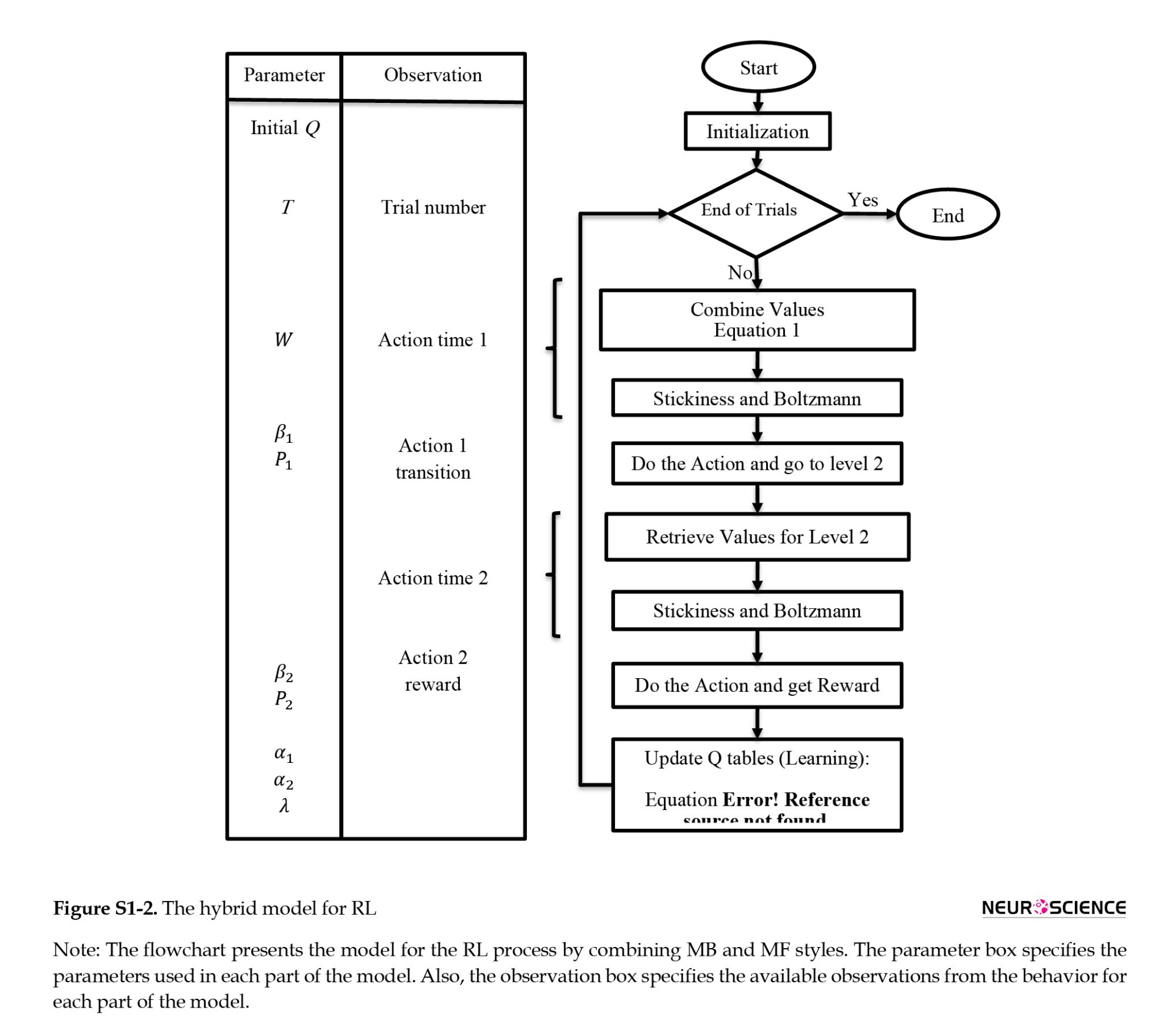
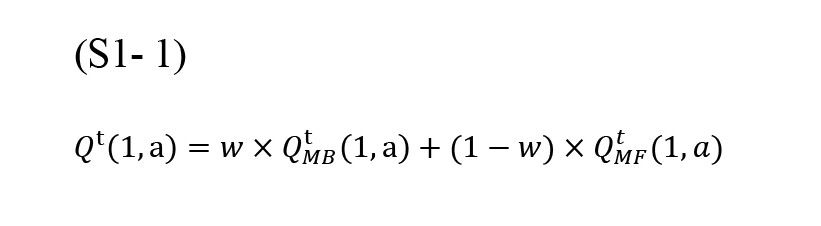
In any trial (t), the value of each action (a) of the first state is calculated by the weighted sum of MB (QtMB) and MF (QtMF) system value (weight: w) according to the Equation S1-1.
the behavior for each part of the model.
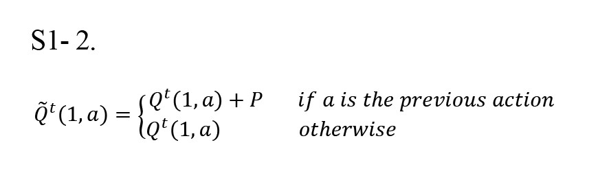
The stickiness increases the value of the previous action for the current trial by adding P to its value (Equation S1-2).
The softmax or Boltzmann machine is a stochastic, biologically plausible approximation of the maximum operation, which is widely used to extract the probability of choosing each action based on its value (Equations S1-3).
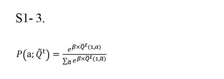
β is the inverse temperature that controls the trade-off between exploitation and exploration. Due to the non-deterministic environment and its probabilistic nature regarding rewards, it is typically assumed to be a fixed parameter across trials but varies across subjects.
In the second stage of the task, the corresponding Q values in each state determine the probability of the chosen action using the same stickiness and softmax equation.
In the beginning, the Q values of all state-actions are initialized to zero, and the update rules (Equation S1-4) change the value of state-actions at the end of each trial. In the second stage of the task, the update rule is the same for both the MB and MF approaches. In the first stage, however, action values are updated using the state-action-reward-state-action (SARSA)-λ method for the MF method. In contrast, the environment model is used to update the QMB based on Bellman’s equation. Note that update rules for QMF are applied only to the performed action, while QMB updates all action-values of the first stage.
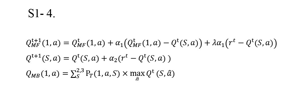
, where PT(1,a,S) is the probability of transition from state one towards the second stage state S, acting a and may be assumed as the real value (i.e. 0.3 and 0.7) or calculated by the Beta-Binomial Bayesian updating rule according to Equation S1-5.
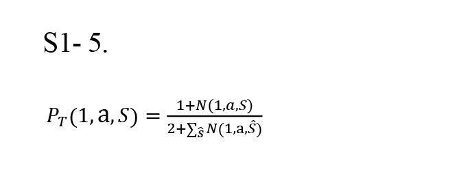
, where N(1, a, S) is the number of transitions from start-state to state S by acting on a. In this study, we calculate the transition probability according to Equation S1-5.
The stop criterion is the fixed number of trials, T, set to 201 for all analyses.
Supplementary 2 (Analyzing the Model Fitting More Precisely)
Effect of agent parameter set in model fitting
Variation of models in model fitting can lead to different error levels, but what about the agent model version? To investigate this effect, we ran 5000 independent agents with different versions listed in the manuscript. For each data set, all model versions, including ML and MAP model fittings, are applied to the observations.
These fittings, as specified by ML and MAP, are summarized in Figure S2-3, parts A and B, respectively. Based on this Figure, when the agent has zero eligibility trace (IS0ENS or DS0ENS), and the fitting method assumes a significant eligibility trace (IS1ENS or DS1ENS), the estimation error is extensive. Also, the error is substantial in reverse situations. The eligibility trace (λ) controls the effect of the second-stage state-action reward on the first-stage action value in SARSA-λ machinery. The λ value strongly affects the behavior of pure SARSA-λ. Therefore, by making a wrong assumption about the λ value, the information about MB-MF in behavior will be confusing and result in a significant error in the w estimation.
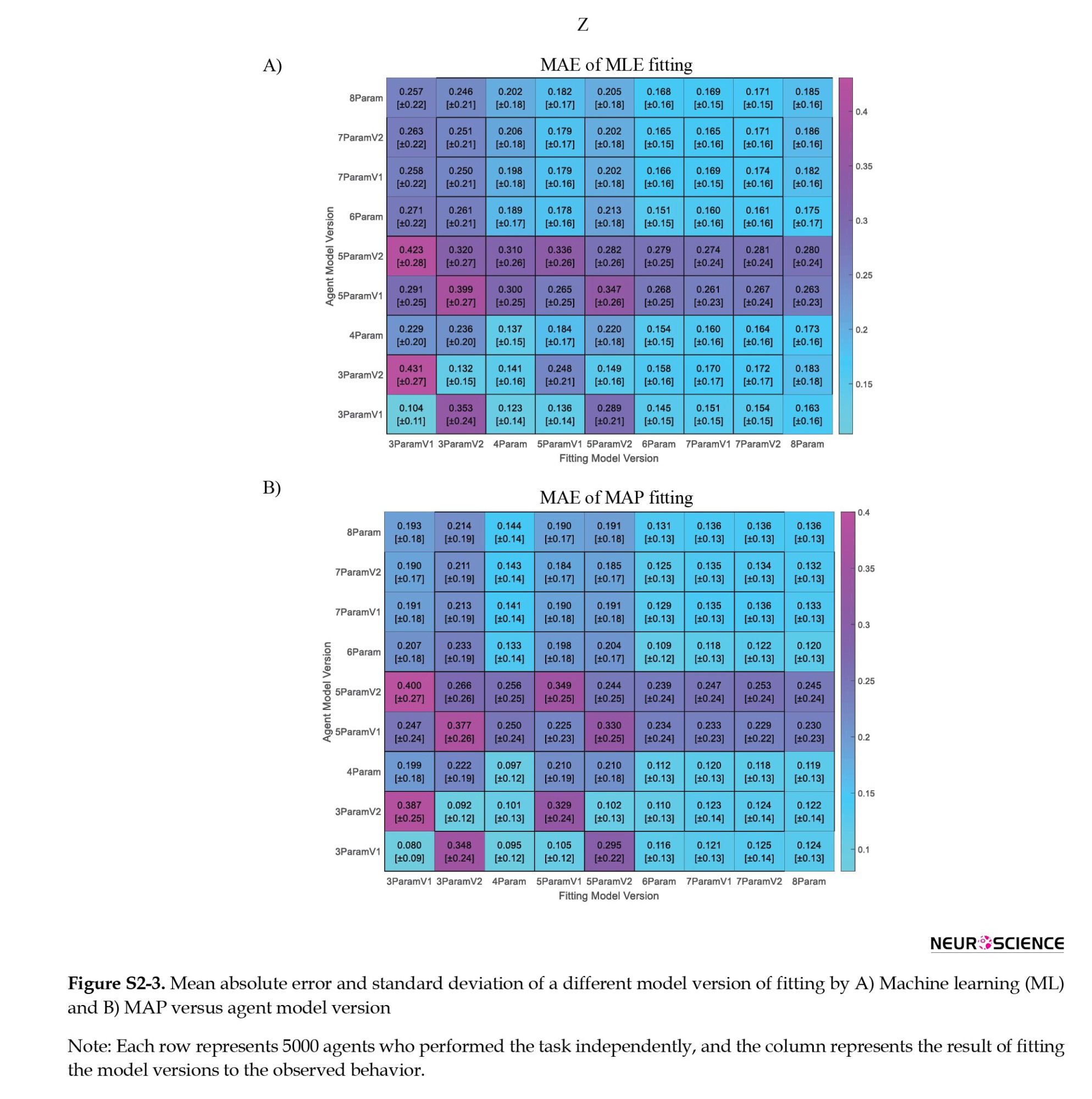
In addition to this remarkable point, knowing the model that the RL agent has used does not always result in a lower error, especially when the model is more complicated. It seems that the randomness of behavior, especially overfitting in the more complex model, causes this point.
Effect of agent learning rate and temperature on model fitting
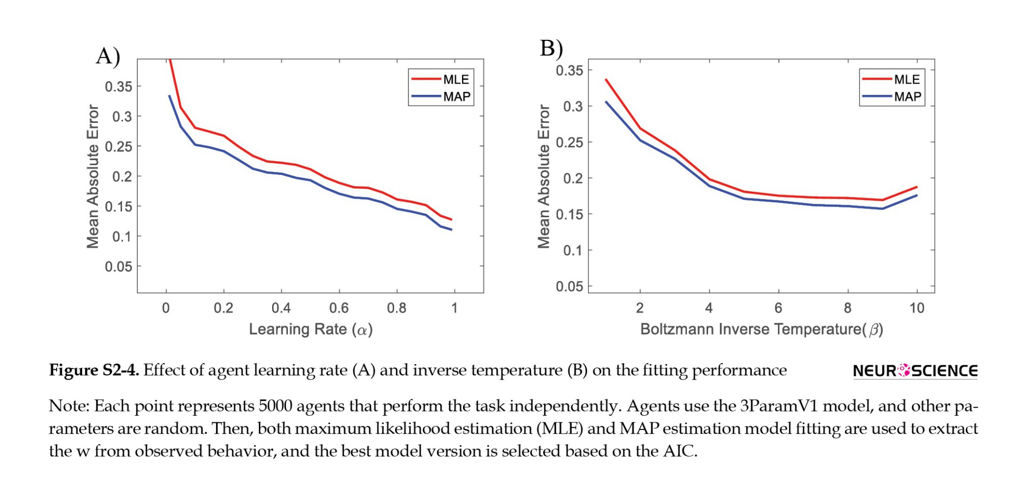
Assume that an agent uses the IS1ENS model while performing the Daw task, and w is extracted by the best model based on the Akaike information criterion (AIC). The question here is whether the parameter’s value in the model affects fitting error. To this end, we run 5000 agents with fixed number sets of learning rate (α) and inverse temperature (β) individually, while all other parameters are sampled randomly.
Figure S2-4 demonstrates the result of this simulation. Figure S2-4, part A, shows that the estimation error is significantly higher at the low learning rate. A low learning rate means that the agent cannot follow the changes in the environment, i.e. the changes in the environment are faster than the low learning rate can track. This agent has difficulty in choice evaluation by both MF and MB styles. This difficulty leads to incorrect decisions that appear random, and model fitting faces additional challenges, resulting in higher error rates.
Figure S2-4, part B, shows that agents with low inverse temperature (β<3) have a high MAE, which decreases for larger β values. A low value of β means more exploration, and similarly, a low value of α results in more behavior that seems random.
The α controls the effectiveness of the new trial in comparison with the previous estimation. Low α values indicate that the previous estimation is precise enough for decision-making from the agent’s point of view. Hence, the new observation for rewarded or unrewarded action changes the evaluation slightly. This small change results in the same behavior on MB and MF systems.
Inverse temperature, on the other hand, controls the exploration-exploitation trade-off. The low β values result in a similar choice probability for actions, regardless of their values, which leads to more exploration. In this case, the effect of the action’s values, calculated by either the MB or MF systems, decreases and is marginally ignored (β becomes zero). So, it is expected that the explorative subject has slight information about the MB or MF system preference, and extracting the subject’s preference towards MB style will be more difficult by any estimation. High β values indicate that even slightly higher values of action make them more preferred choices, suggesting exploitative behavior. For high β values, either little or huge differences in action-values have the same effects on the behavior.
Supplementary 3 (k-NN Estimation)
k Nearest neighbor estimation
For numerous observations, assume that we have an exact value of the combination weight of MB/MF learning styles (wo). The feature vector is extracted from each observation, and these feature vectors, along with their related well-known value (also known as the label), are stored in a database. By having this database, we want to estimate the combination-weight for newly observed behavior data (ŵk-NN). Based on this data, the feature vector was calculated, and then we linearly normalized this vector in the feature space (Equation S3-1).
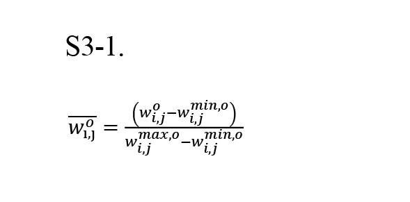
Where woi,j, wi,jmin,o and wi,jmax,o are the value, minimum, and maximum of the observed feature vector in the jth dimension of the ith agent, respectively. Then, we calculate the Euclidean distance (d) of this feature vector from other vectors in the feature space and find the k nearest features based on d. Now the estimated value of the combination weight for this observation is given by Equation (S3-2):
S3-2.
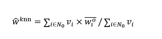
, where wioɛ[0,1] is the label of the ith sample in the dataset, and N0 is the index set of k nearest neighbor, and Equation S3-2 calculates the weighted factor vi.
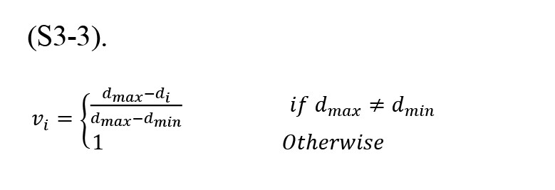
, where in Equation (S3-3), dmax and dmin are the maximum and minimum distance values of the neighbor, respectively.
The feature space and hyperparameter k have the most impact on the results. The k parameter controls the localization and generalization of the k-NN learning method and has an optimal value. To achieve the best k-nearest neighbor performance, we adapt the k value by exhaustive search to minimize MAE. Based on the analysis, when k is greater than 30 and up to 100, the MAE is nearly constant. For these values of k, the MAE varies minimally, ranging from 0.1943 to 0.1948. However, the optimal value of k is 69, which we use in all different situations.
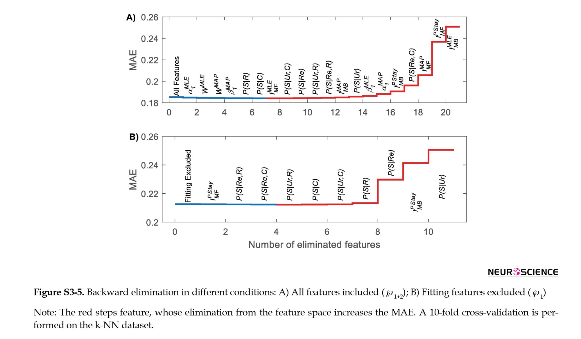
In addition to the k parameter, the feature selection can improve k-NN performance. To optimize the feature space, we used the backward elimination algorithm. Backward elimination begins with all features, and in each step, the best performance is achieved by eliminating one feature. These steps continue until all features have been eliminated or any other features make no improvement. We use backward elimination in two conditions based on available features (℘1+2 and ℘1). Based on Figure S3-5, the improvement in MAE is very low (<0.001), indicating that all introduced features are likely beneficial. We also check the linear correlation between all pairs of features, and all relations are below 0.95, so we cannot eliminate any feature using unsupervised feature selection. Due to low improvement, we ignore the feature selection in the paper.
Supplementary 4 (Behavioral Analysis of Gaze Data)
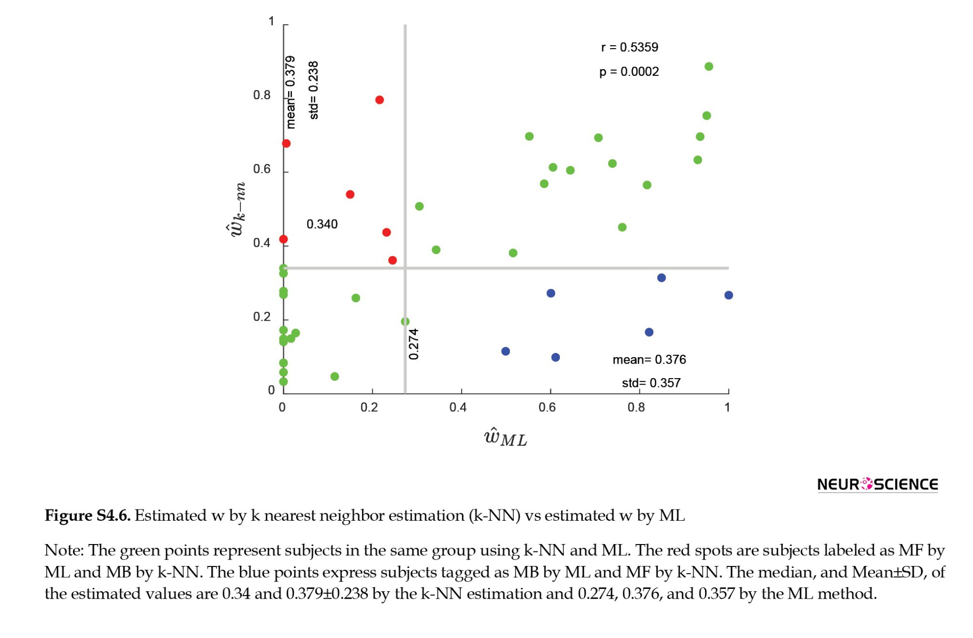
We investigate grouping by using the mean value of P-Stay in groups as a behavioral indicator. When the ŵk-NN instead of the ŵML was utilized, several subjects’ groupings altered, as shown in Figure S4.6.
The first question concerns which groupings are more consistent with behavioral observations. To answer this question, we extract the stay probability from distinct groupings and subjects with different labels (Figure S4.7).
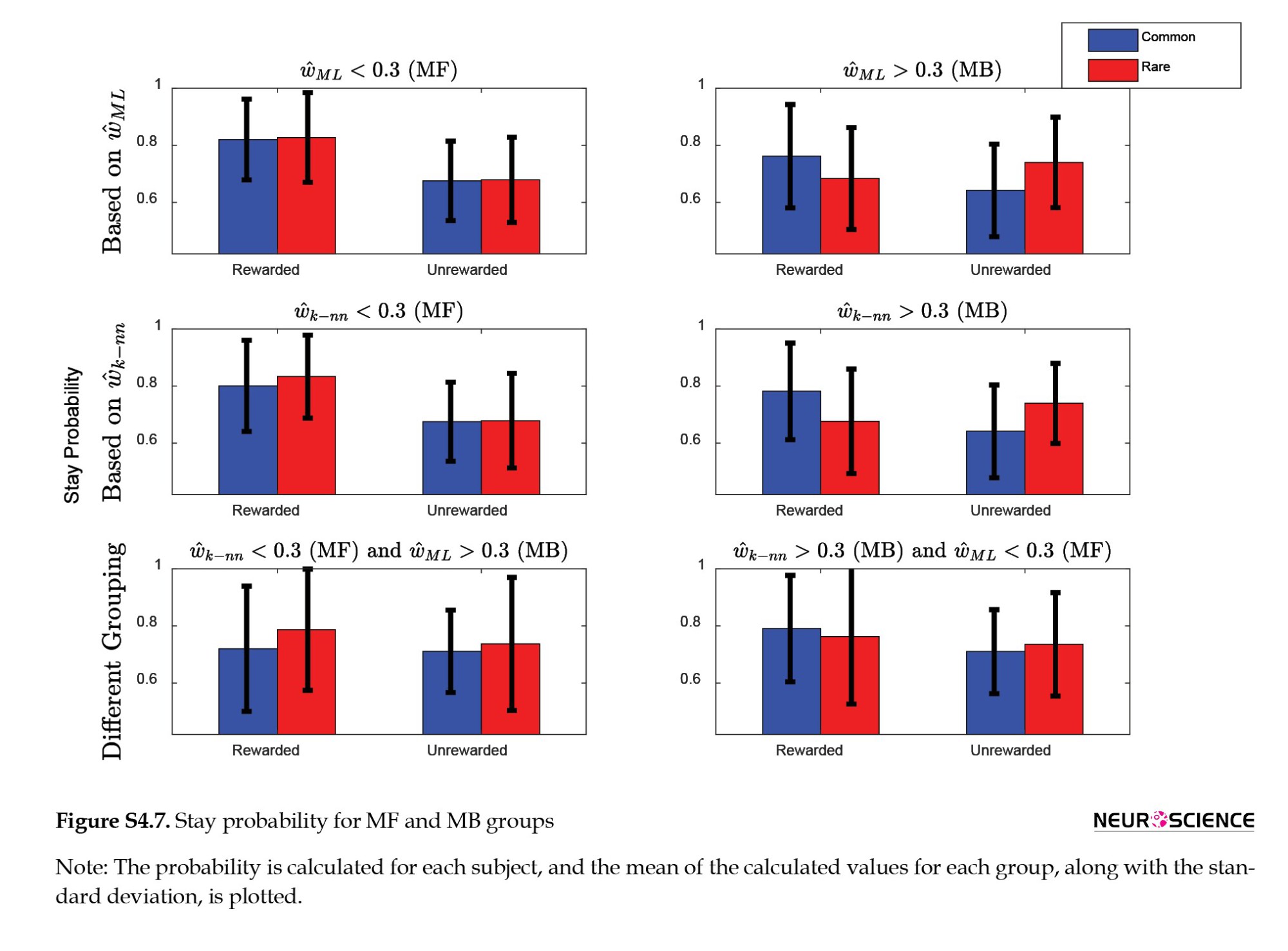
According to Figure S4.7, ML and k-NN are both consistent with previous findings. For subjects categorized as MB by ML and MF by k-NN (the blue subjects in Figure S4.6), the stay probability in trials after rewarded trials is higher than the stay probability in trials after unrewarded trials in different transition conditions (common or rare transitions in previous trials). This behavior is caused by ignoring the transition, which is the primary specification of MF subjects. As a result, these subjects are better candidates for the MF label than the MB label, and consequently, the k-NN outperforms the ML. The stay probability demonstrates attention to the transition for subjects designated as MB based on ŵk-NNbut MF on the basis of ŵML (red subjects in Figure S4.6). As a result, these individuals are stronger candidates for the MB label than the MF label, and hence the k-NN outperforms the ML.
Full-Text:
Introduction
Multiple cognitive systems are thought to control human decision-making. Most decision-making and learning occur during a person's lifespan as a result of habitual and goal-directed systems (Dolan & Dayan, 2013; Wanjerkhede et al., 2014). The habitual system fosters habits and automatic decisions, whereas the goal-directed system is primarily concerned with planning and making decisions. Researchers studying reinforcement learning (RL) assign habitual and goal-directed systems to model-based (MB) and model-free (MF) learning styles. The only distinction between the MB and MF styles is in the evaluation of state-action. In MB learning, an environmental model is used to evaluate each decision in the current state. In MF learning, action values update without the use of any explicit environment model, and the value of each action in each state is learned via trial and error.
Previous studies found that people employ a combination of MB and MF learning to direct their behavior during learning tasks. Several studies support the notion that the hybrid model is an effective subject description (Daw et al., 2005; Dolan & Dayan, 2013; Gijsen et al., 2022; Keramati et al., 2016; Kool et al., 2016; Lucantonio et al., 2014; Toyama et al., 2017). The combination weight (w) is the parameter that affects the subject's preference for MB in this model, as explained in Supplementary 1 (Daw et al., 2011).
Computational models can assist in extracting various cognitive components that drive maladaptive behavior, and the model parameters associated with those components can be utilized to investigate the potential sources of cognitive deficiencies (Ahn & Busemeyer, 2016).
One of the elements that can be used to analyze, diagnose, and evaluate the efficacy of therapies for psychiatric diseases is the parameter that determines the subject's preference for the MB/MF style (Montague et al., 2013). In a two-stage task proposed by Daw et al. (2011) the reward probability in the second stage fluctuates over time, and the transition from the first stage is probabilistic. As a result, the MB and MF styles behave differently. Researchers frequently use this task to determine how much participants prefer MB and MF styles (Daw et al., 2015; Doll et al., 2015; Feher da Silva & Hare, 2020; Foerde, 2018; Gillan et al., 2015; Miller et al., 2022; Morris et al., 2017; Otto et al., 2013; Smittenaar et al., 2013).
Considering changes in the subject’s preference toward MB (w) due to pharmacological or cognitive manipulations or neuropsychiatric conditions will provide important insights for clinical research. For example, over-reliance on the MF style could lead to inflexible decisions in addiction and compulsion (Everitt & Robbins, 2005; Gillan & Robbins, 2014; Lucantonio et al., 2014). Some studies show that patients with obsessive-compulsive disorder (OCD) prefer the MF learning style more than MB (Gillan et al., 2011; Gillan & Daw, 2016; Toyama et al., 2019; Voon et al., 2015). Wit et al. (2011) demonstrated that mild Parkinson disease leads to impaired motor habit formation. Also, Culbreth et al. (2016) reported that in schizophrenic patients, MB behavior is low. On a broader view, there is a growing consensus that computational modeling can be a constructive approach to understanding psychiatric disorders. Therefore, reliable and precise estimation of the w is important for many applications. However, reliable estimation of parameters is a challenge due to noise in behavior, confounding factors, and a low sample size, especially for extreme values.
Traditionally, researchers have estimated model parameters, such as the subject's preference for MB (w), by fitting the model to their observations using maximum likelihood (ML) or maximum a posteriori (MAP) methods. The best objective function for model fitting is the likelihood when no other information is available beyond behavioral observations. The foundation of ML is the notion that a specific collection of parameters has a greater likelihood of being responsible for the observed data. ML is widely applied in the behavioral sciences (Ward et al., 2012). Additionally, if we are aware of any prior knowledge about parameters, we employ the MAP approach.
According to the analysis, the precision of the estimated w based on conventional model fitting is subpar. The precision of traditional methods is affected by factors such as the nature of the task, the model, noise, the fitting process, and the limited number of observations. Our simulations demonstrate that the conventional estimation technique is biased toward the MF style, particularly when the other model parameters are outside the acceptable range. In model fitting, the estimation of the w is more inaccurate when the learning rate or temperature is low or high, respectively (Supplementary 2).
In the present research, we propose that incorporating a data-driven learning method alongside traditional fitting methods can enhance the precision and reliability of estimation. This research employs the k-nearest neighbor (k-NN) algorithm as a straightforward learning technique (Supplementary 3). Other learning algorithms, such as deep neural networks, can serve the same function. Although this study focuses on observing action selection, the estimator can be made more precise by incorporating other measurable parameters, such as confidence level or response time (Shahar et al., 2019).
In this study, we aim to enhance the estimation of a model's parameters based on behavioral observations, as compared to the traditional methods. Although we analyze the effect of some nested models on parameter estimation error, we do not investigate which model is superior in other ways, such as predicting human behavior. This study did not examine alternative models, such as the Gijsen model (Gijsen et al., 2022). Some studies use the reparameterization method (alternative models with different free parameters) or other combinations of reparameterization (Gillan et al., 2016; Toyama et al., 2019). In addition, some studies utilize the response time of a model that is unavailable for our simulation and was not incorporated into the model (Shahar et al., 2019). Although a subject's preference for a particular style can change over time, we will assume that it remains constant for the duration of the task.
Methods discusses the basic model architecture (section 2.1) and the k-NN estimator (section 2.2). Sections 2.3 and 2.4 explain implementation. Section 3 sets the k parameter (section 3.1) and analyzes the results of the proposed method (section 3.2). Section 3.3 examines the w extraction in a noisy model. Section 4 presents the experimental performance of the k-NN method and its advantages. The conclusion discusses the proposed method and summarizes the results (section 5).
Materials and Methods
In this study, we compared the results of determining preference for MB (w) using the traditional method and the proposed method for both humans and simulated agents. In the simulation and ML/MAP methods, we employ the Daw et al. (2011) model (Supplementary 1). During the training and testing phases, the behavioral data are derived from simulation, whereas during the recall phase, it is derived from actual human behavior. Figure 1 illustrates the proposed method in its entirety.

In this paper, in addition to the estimated values of the parameter obtained by ML or MAP, we utilize global information, including behavioral statistics and indices, to extract the subject's preference for MB (w) more precisely. In the proposed method, the k-NN estimator (also known as the k-NN regressor) is employed as a learning system to extract w from behavior. k-NN is a supervised, nonparametric learning method that has been widely adopted as an accurate point estimator (Li et al., 2017). The w parameter is estimated by k-NN using a set of labeled feature vectors. To train the k-NN, we employ simulations of RL agents, and the dataset is populated with features derived from observations labeled by the agent's w parameter (wo).
Since we know the parameters of the RL agent during the testing phase, the estimation error can be calculated. We illustrate the error distribution using the mean absolute error (MAE) as a point estimator of the error and the standard deviation (STD). The simulations contain a sufficient number of agents to yield reliable results; therefore, the statistical test results are not reported for the simulation data.
In the current study, the objective functions are minimized by the interior-point optimization algorithm, and 10 random starting points are used to maximize the probability of global optimization for ML and MAP. All analyses and optimizations have been implemented in MATLAB software, version 2021b and are accessible via the Dataverse repository.
In the training phase, the simulated RL agent performs the task, and in the recall phase, observed data from human behavior is utilized.
Computational model
Daw et al. proposed a computational model predicated on the notion that subjects utilize both MB and MF learning styles, with the values being linearly combined. They suggested using the SARSA λ algorithm to extract the MF style value and the Bellman Equation to extract the MB style value. Using a linear weighted combination, the net value of an action (a) in a state (s) is computed for each trial (t) (Equation 1).

The free parameter w represents the subject's MB learning style preference. Then, the value of the same previous action increases by the stickiness parameter (p), and the model extracts the probability of decisions using the softmax function. Each trial is updated by incremental learning, which modifies the state-action values (Supplementary 1). Multiple other researchers have also employed this hybrid model (Kroemer et al., 2019; Morris et al., 2017).
The Daw model for the task contains 7 parameters (DS-λE-SS), but in many studies, some of these parameters are set identically in two stages or are assumed to have a constant value. We extracted nine model versions for analysis using this method. The models and subsets of each version's parameters are detailed in Table 1.
k-NN
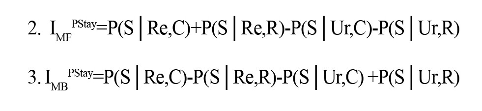
The distance-weighted method of the k-NN estimator is utilized. T groups of behavioral observation-derived characteristics are listed in Table 2. There are 10 characteristics within each group. The first set is based on the stay probability, which is calculated by counting the number of stays in observed behavior, i.e. selecting the same action as in the previous trial in the first stage. Numerous studies utilizing the Daw two-stage task employed the conditional stay probability for analysis (Collins et al., 2017; Daw et al., 2011). We estimate the stay probability across situations and conditions based on the reward value (either rewarded or unrewarded) and transition frequency (common or uncommon) of previous trials. In addition, the slope of stay probabilities, as an index for MF (Equation 2) and MB (Equation 3) behavior (Miller, was utilized as an additional behavioral indicator in feature space (Miller et al., 2016).
The second group consists of model-parameter-using and model-fitting features. Miller et al. (2016) introduced the MB/MF preference indexes, as outlined in equations 4 and 5, which we employ.
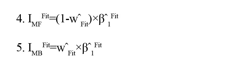
In these equations, ŵ and β ̂1 are the w and inverse temperature of the first stage, respectively, and are derived by fitting the model using ML or MAP. In addition, we include some RL model parameters, such as the w itself, which is estimated by fitting the model using ML or MAP (Supplementary 3).
Generated dataset for k-NN
As a supervised learning technique, k-NN requires a training dataset with the appropriate labels to perform properly. Therefore, we simulate 80000 independent RL agents with random parameters and the DS-λE-DS version (Table 1), and then record their behavioral observations. In this study, we selected all random parameters and MAP prior knowledge as listed in Table 3. Each simulation includes a series of trials and associated observations, all of which are tagged with the wo. In addition, 10-fold cross-validation is utilized to tune the hyper-parameter k. To eliminate estimator bias at extremes, we augment the training dataset with 10000 MB and 10000 MF agents.
Model the lapse in decision-making
It has been demonstrated that incorporating the lapse rate into models for human subjects can increase the quality of fit for numerous psychophysical paradigms (Wichmann & Hill, 2001). This lapse rate is a result of the participant's participation in random and unattended trials. We add this noise source capability for agents in simulations. Each agent's choice is reversed based on a probability known as the lapse rate or noise level. We simulate the noisy model with varying lapse rates in the interval [0, 0.5].
Results
In this section, we will begin by setting the k parameter of the k-NN algorithm. We will then apply the necessary statistics and visualizations to demonstrate the effectiveness of the suggested technique. According to the findings of the analyses, both the variance and the bias of the estimation decreased.
k-NN parameter
The value of k affects the effectiveness of k-NN. The value of k determines the localization and generalization of k-NN, and a trade-off between these two factors is required for optimal performance.
To achieve the best k-NN performance, we optimize the k value using exhaustive search to minimize MAE. Experimentally, the MAE is nearly constant when k is greater than 40 and less than 100. The MAE varies minimally within the range of 0.1857 to 0.1862 for these values of k; however, the optimal value of k is 69, which we use in all situations.
Feature selection can improve k-NN's performance. We used both unsupervised (analyzing feature correlation) and supervised (Backward elimination method) feature selection on the dataset; however, the performance improvement was minor, so we ignored the feature selection (Supplementary 3).
As mentioned previously, Table 2 contains two feature groups. The first group of features is calculated based on the stay probability. The second group of features requires the fitting procedure, which is complicated by computational load, model selection, and optimization algorithm. To adjust the proposed method for some practical applications in which the mentioned factors restrict the use of fitted parameters, we can disregard the second group of features and, as a result, decrease the method's performance (although in some cases, like having not a good model or noisy observation, this neglecting can improve the performance). We utilized k-NN in two distinct circumstances based on the available data and analytics:
℘1: Just first group available (features from model fitting are excluded)
℘1+2: All features will be computed (needs model fitting, i.e. ML and MAP estimation).
Performance
Figure 2 depicts the scattering of the extracted w by the k-NN estimator and traditional model fitting relative to the corresponding value of agents. To have a clear view, we have divided it into 5 areas. We are aware that the exact combination weight (wo) cannot be determined due to limited data, so a small error is acceptable. We assume an error of less than 0.1 is tolerable. Grouping subjects by learning style is an application of extracting the w. Therefore, if an error in w extraction results in the incorrect subject label, the error is considerable. The areas that were not altered by the dominant strategy are considered slight errors.
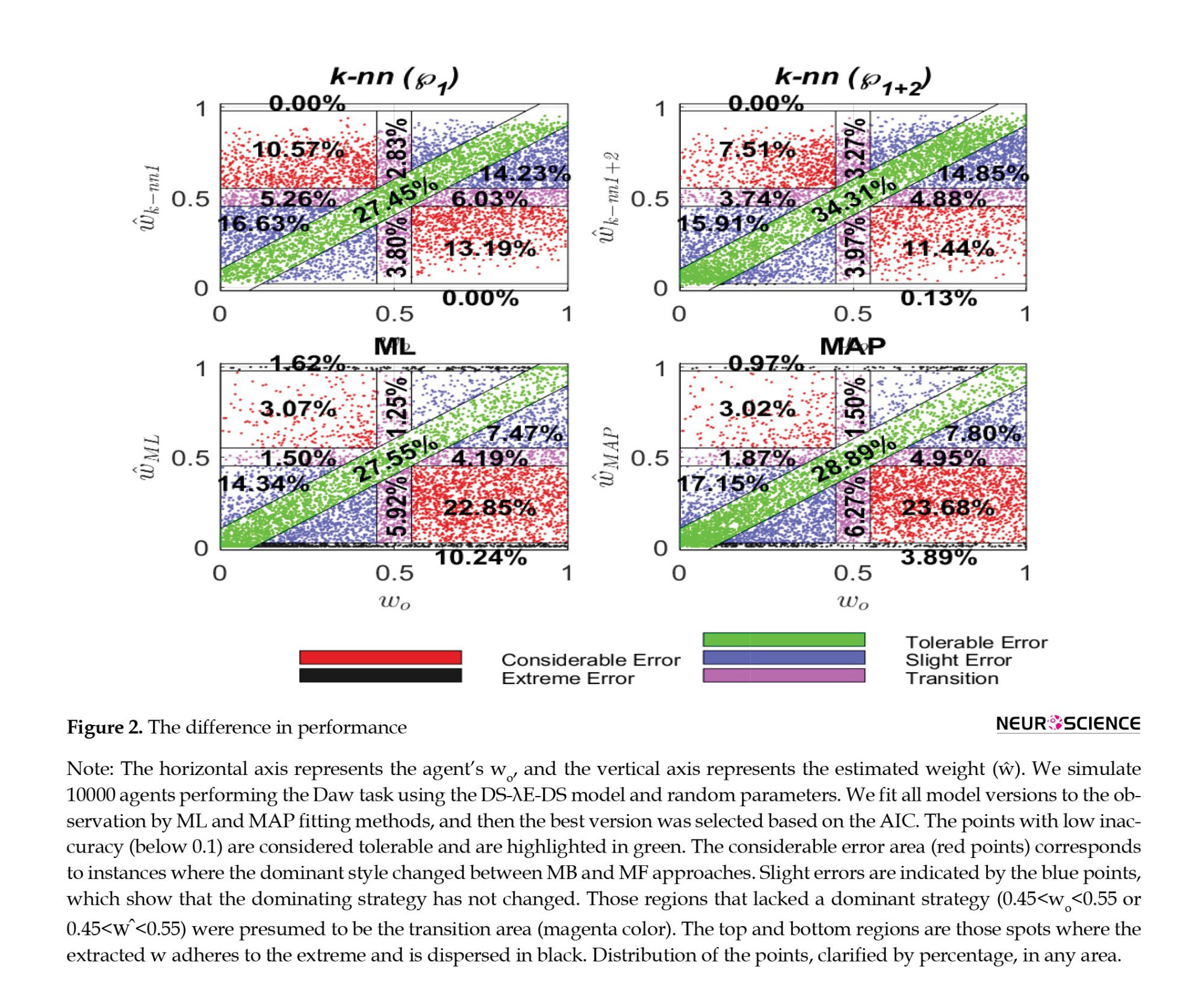
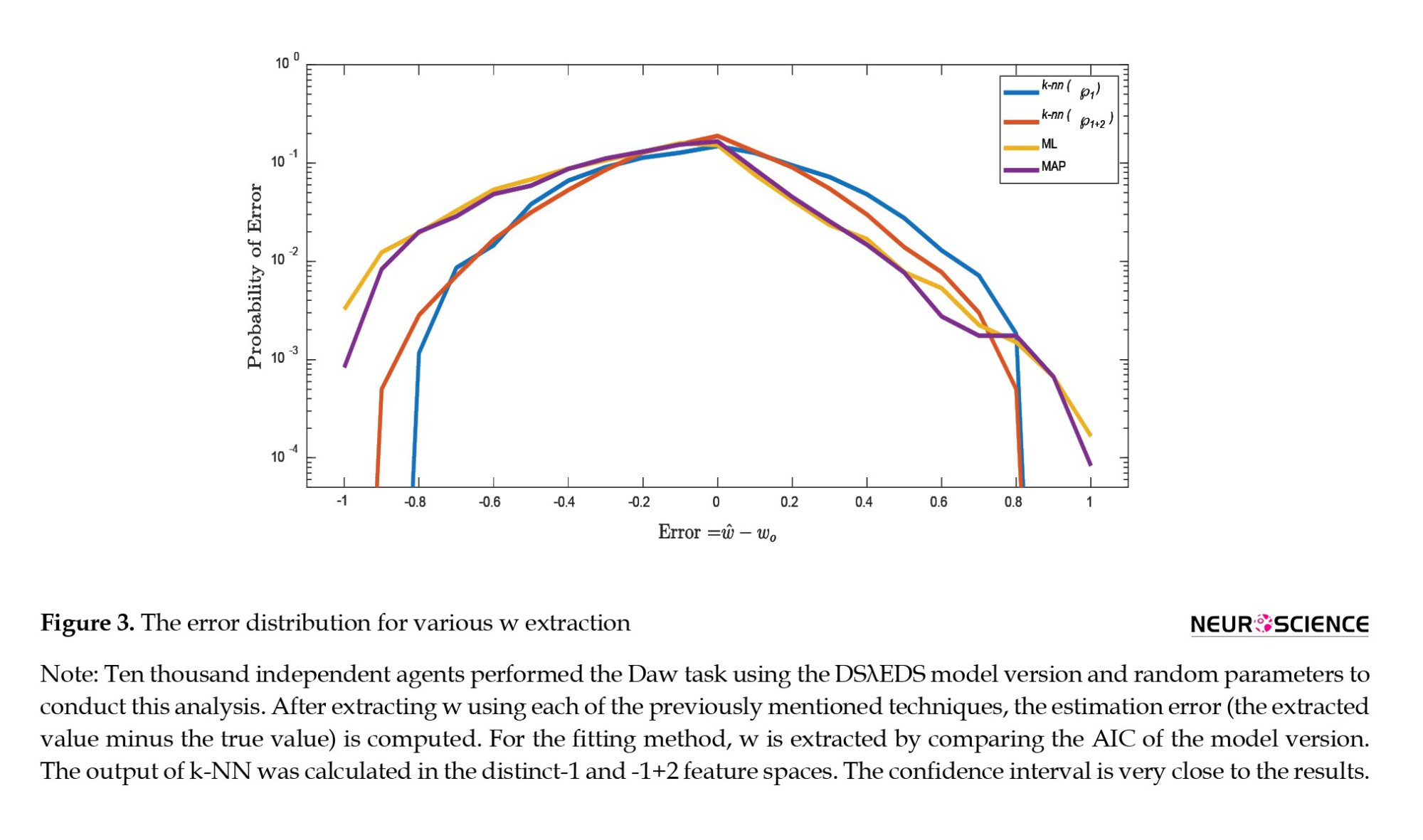
Those zones without a dominant strategy (0.45 Individual difference is an important issue, especially in computational psychiatry. In many cases, the percentage of high error is more important than the exact estimation; in other words, it is crucial to have an estimate with low error variance. Figure 3 illustrates the distribution of error, which is the difference between the estimated and true values.
Figure 3 demonstrates that the k-NN technique reduces both bias and variance of error. For the k-NN approach, the tail of the distribution consists of lower values. The standard deviation of errors confirms that the k-NN error variance is superior to that of traditional methods (Table 4). In contrast, the chance of tolerable error (errors between -0.1 and 0.1) is greater for k-NN approaches than for fitting methods. In addition, Table 4's presentation of the MAE and correlation coefficient demonstrates that the k-NN estimation reduces bias and error variance. Extreme errors are substantially more in ML and MAP than in k-NN-based algorithms. Since extreme values for the subject's preference for MB and MF styles are possible under clinical situations, these regions are significant. k-NN approaches correct these errors and make the clinical trial model more robust. In accordance with Toyama's work, the skewness of the error in Figure 3 indicates a bias toward MF (Toyama et al., 2019).
Lapse in decision-making
The potential of erroneously selecting the desired option due to attentional lapses or other issues is a real concern in parameter estimation for human data. When considering the effectiveness and applicability of an estimation technique, we should consider its resilience in the face of lapse rates.
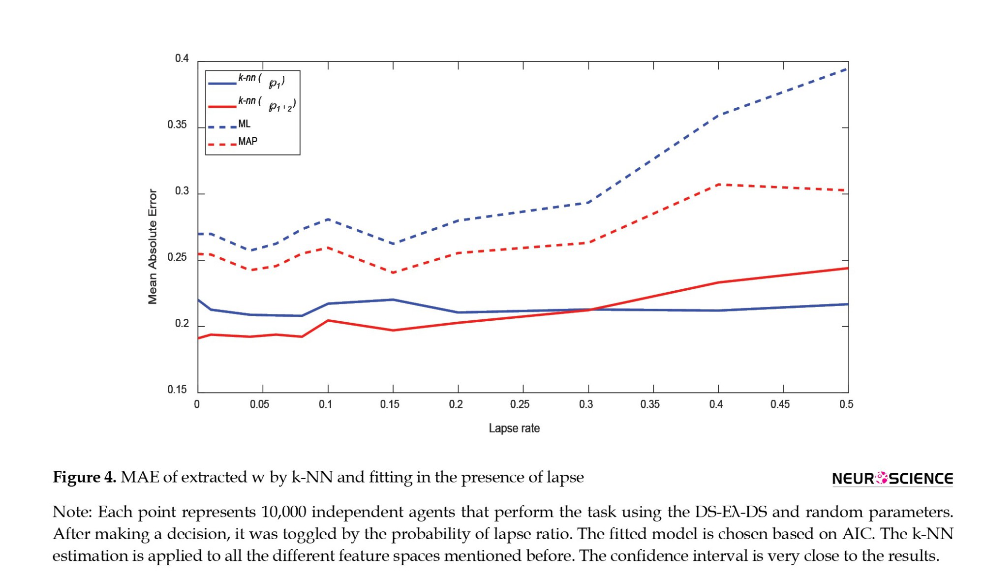
We simulate the model with different lapse rates to see what happens when people make mistakes. Figure 4 illustrates the differences between the k-NN estimation method and traditional methods of fitting.
Based on Figure 4, it is clear that k-NN methods are more resistant to lapse than traditional fitting methods, especially when feature-based features are removed from the feature space.
Experimental data analyses
This section validates the proposed method using actual experimental data. To validate the proposed method, data from two independent studies were chosen. The comparison of results based on "w from the proposed approach" (ŵk-NN) to results based on "w from traditional methods" (ŵML or ŵMAP) demonstrates the superiority of the proposed method.
Analysis of the relationship between learning style and gaze direction
Using the Daw task, Konovalov and Krajbich (2016) have already investigated the correlation between gaze information and the w. They used the Daw task in two ways, and we use the first one to make sure our models are the same. ML has used the IS λE SS version of the model to get the w value (Table 1). In this study, we used the k-NN estimation with ℘1+2 feature space to extract the w from their data. The number of trials in the Konovalov study (2016) has been set to 150, so we make a different database by setting the number of trials in simulations to 150.
Konovalov and Krajbich divided subjects into two groups based on the median of ŵML (0.3) to study the differences between MB and MF behavior. When the ŵk-NN instead of the ŵML was utilized, several subjects' groupings were altered. We first focus on the behavioral differences in the sense of stay probability across different groups, and we observe that subjects in the traditional method and proposed method have conflicting groupings. The analysis indicates that the traditional method divides the subject more effectively than the traditional one in terms of stay probability (Supplementary 4).
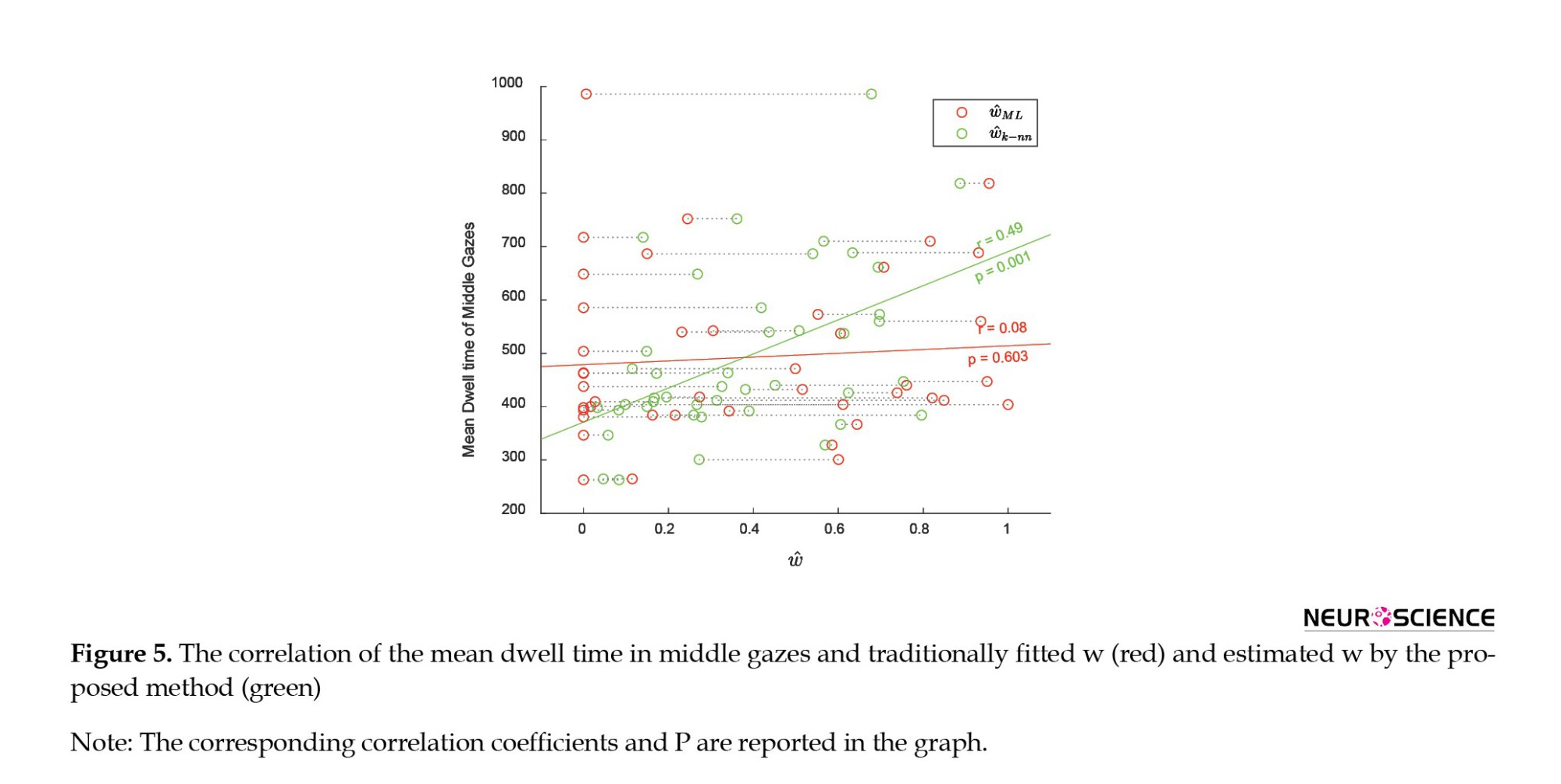
We validate all of the studies presented in the first part of the paper by Konovalov and Krajbich (2016) using k-NN group labels. While the major analytical results remained unchanged, a notable relationship was observed. We examined the correlation between ŵk-NN and all behavioral data of subjects. There was no correlation between ŵML and available significant behavioral indices not mentioned in the paper. But using the proposed method, we observed that the mean dwell time in middle gazes was strongly correlated with ŵk-NN (correlation coefficient=0.5, P=0.001). In contrast, the ŵML and the mean dwell time of middle gazes were not correlated (correlation coefficient=0.08, P=0.603). Figure 5 depicts this amazing association.
The proposed method reveals information from the data that would have been overlooked if traditional fitting methods were used. This information did not alter the results of the Konovalov and Krajbich study.
Analysis of the relationship between learning style and symptom dimension
Gillan et al. (2016) used the Daw task to examine the relationship between learning style and compulsive behaviors. While they utilize the Daw task without modification, their analytical model differs from the task itself. Their computational model is a modified version of the reparameterization model presented by Otto et al (2013). They demonstrated strong correlations between certain psychiatric diseases and the subject's preference for MB style. However, these correlations for the w are absent due to imprecise estimation in conventional fitting methods Table 6. We believe a more accurate estimation strategy can revive these relationships in the Daw et. al. (2011) model.
To ensure a fair comparison, we conduct the same analysis as Gillan et al. (2016), but with the model version assuming DS-λE-1S instead of a modified reparameterization model. We use traditional fitting methods and the proposed method to extract ŵ. Table 6 reports the correlation between subject aspects and reports. Table 6 reports the regression analysis between the total scores of the self-report questionnaire and ŵ.
As a control for regression analysis, Gillan et al. used age, IQ, and gender, which have been previously reported to covary with goal-directed behavior (Eppinger et al., 2013; Gillan et al., 2016; Schad et al., 2014). In line with the Gillan et al. (2016) study, the extracted w by k-NN methods shows significant relationships with age, IQ, and gender. Still, only a relationship exists between age and ŵML (Table 6). The traditional fitting method extracts the ŵ that is inconsistent with other analyses, such as some studies (Eppinger et al., 2013; Schad et al., 2014).
Based on one-trial-back regression analysis in the Gillan et al (2016) study, there was a significant inverse association between goal-directed behavior and scores on the eating disorder, Impulsivity, OCD, and alcohol addiction questionnaire (Table 6). The k-NN methods replicated some of this association, but the traditional fitting methods did not. The k-NN (℘1+2) replicates the association between goal-directed behavior and the score of OCD and alcohol addiction. Also, the k-NN (℘1) method replicates the association between goal-directed behavior and the score of impulsivity and alcohol addiction (Table 6). On the other hand, the MAP method replicates an association between goal-directed parameters and apathy score, which is not in line with other studies and regression analyses.
Gillan et al. (2016) introduced three factors for further analysis, and we also analyzed the correlation between these factors and extracted ŵ by different methods. The regression analysis reveals a significant association between factor 2, ‘compulsive behavior and intrusive thought,’ and goal-directed behavior (β=-0.046, SE=0.01, P<0.001). The proposed method also replicates this relationship, but the traditional fitting methods missed it. Moreover, there were no significant effects of factor 1 (β=-0.001, SE=0.01, P=0.92) or Factor 3 (β=0.013, SE=0.01, P=0.24) based on both regression analyses and the proposed method; however, the traditional fitting method reported an association.
The proposed method could replicate some relationships between goal-directed behavior and some psychiatric disorders, but traditional fitting methods missed this relationship. This issue may be due to the noise reduction achieved by the proposed method compared to traditional fitting methods. Note that Gillan et al. (2016) show these relationships by regression and a different model. Therefore, we can conclude that this estimation method is more reliable than traditional methods in identifying clinically relevant relationships.
Discussion
The MB and MF learning balance extraction is necessary for transitioning RL modeling to mathematical psychology. The Daw two-step task was designed to differentiate between MB and MF learning styles and was widely used. We studied the precision of extracting the subject’s preference towards MB style utilizing this task. We used 9 nested versions of the model. To establish a performance measure, we observed the simulated model's behavior while performing the Daw task, and then extracted the w from the observed behavior.
Our analysis revealed that the complex model overfitted the observations, and simple models with erroneous assumptions resulted in higher errors (Supplementary 2). Moreover, when prior knowledge was not assumed for the fitted parameters, the fitted values sometimes stuck to the extremes of the parameter range. Our analysis shows that the agent parameter also affects the error. MB and MF styles have similar behavior when the learning rate or inverse temperature is low. In these conditions, the estimation error increases (Supplementary 2). Such problems in model fitting make the fitted parameters unreliable (Eckstein et al., 2022).
In addition to the traditional model fitting, several statistical indices were extracted and utilized to analyze cognitive studies using the behavioral data. We propose to fuse these two types of information by using k-NN as a simple learning method. Additionally, behavioral information alone can be used to learn parameter estimation instead of model fitting. We use 20 features (including fitting-based features) to generate the k-NN dataset, and then we extract two different feature spaces by eliminating the fitting-based features. Eliminating the fitted-based features reduces both computational load and noise effect. The best performance was reached by k-NN. Both bias and variance of error were proven to be decreased by k-NN learning compared to traditional model fitting. The analysis also specifies that the k-NN method is more stable in the presence of lapse, especially when excluding all fitting-based features. When we use fitting-based features, we encounter model fitting problems, such as low sample size, selecting a suitable model, choosing an effective optimization method, and determining the appropriate objective function. Therefore, if we have no information about the model or fitting, it is better to ignore the fitting-based features. The proposed method is advantageous due to its lower error for extreme cases. Such extreme cases may be prevalent in clinical trials and psychiatric conditions, making the proposed method superior to model-fitting approaches in terms of performance. MAP estimation is better than ML in extreme values because using a prior, k-NN method works better than MAP. The mentioned improvements will enhance the applicability of the Daw task for computational psychiatry purposes.
It was indicated that using the proposed method can help identify a significant correlation between w and mean dwell time, which is not present in the traditional method. It was proven that consideration of behavioral parameters in the estimation of w (in addition to fitting) improves the consistency of behavior and subjects grouping, so other conclusions from this grouping can be more precise. Using the proposed method on clinical subjects has revealed some relationships between disorders and the habitual vs goal-directed behavior axis that were previously missed by traditional fitting methods. These relationships were validated by a reparameterized model and a generalized linear mixed model in Gillan et al.'s (2016) study. Because adding noise to one variable can destroy the correlation coefficient between that variable and other measures, some correlation coefficients have lost their significance due to the noisy estimation of combination weights. The proposed method was more successful due to the reduction of this noise. It is worth noting that, although the proposed method successfully extracted most relationships from the Gillan et al. (2016) study, some relationships were missing, even with k-NN. For example, there was an association between OCD and goal-directed behavior based on regression analysis, but none of the extraction methods reflect that.
Note that any model fitting minimizes an objective function to extract the behavior under different assumptions. The ML maximizes the likelihood function, whereas the extracted parameter by k-NN will not maximize the likelihood, although the estimation error in k-NN is lower. The flow of probabilities in reinforcement agent decisions causes a specific parameter not to guarantee ML, while another parameter exists that satisfies the maximized likelihood criterion. Although ML can theoretically achieve the Cramer-Rao lower bound, the above statement is the reason that learning yields better estimations than ML. The proposed method can be considered a ML estimation using simulation-based estimation. Such a method utilizes trial-by-trial observations of the behavior and global observations, such as stay probabilities in random variable space. It attempts to maximize the likelihood of observing all the mentioned behaviors together. ML and k-NN methods may converge to the same estimation error for large sample sizes. However, for limited sample sizes, k-NN has shown greater reliability and avoids overfitting, making it a better option in typical experimental conditions.
Conclusion
In summary, our proposed method can enhance the estimation of combination weights for both MB and MF approaches. This improvement is due to the use of behavioral indices from the data, which makes the analysis more robust. This robust estimation can facilitate the handling of similar paradigms in clinical applications and aid in the diagnosis of psychiatric disorders.
Ethical Considerations
Compliance with ethical guidelines
There were no ethical considerations to be considered in this research.
Funding
This research did not receive any grant from funding agencies in the public, commercial, or non-profit sectors.
Authors' contributions
All authors contributed equally to the conception and design of the study, data collection and analysis, interception of the results and drafting of the manuscript. Each author approved the final version of the manuscript for submission.
Conflict of interest
The authors declared no conflict of interest.
Acknowledgments
The Authors want to express their gratitude to Arkady Konovalov and Ian Krajbich for sharing the gaze task data with them, and to Gillan et al.
References
Multiple cognitive systems are thought to control human decision-making. Most decision-making and learning occur during a person's lifespan as a result of habitual and goal-directed systems (Dolan & Dayan, 2013; Wanjerkhede et al., 2014). The habitual system fosters habits and automatic decisions, whereas the goal-directed system is primarily concerned with planning and making decisions. Researchers studying reinforcement learning (RL) assign habitual and goal-directed systems to model-based (MB) and model-free (MF) learning styles. The only distinction between the MB and MF styles is in the evaluation of state-action. In MB learning, an environmental model is used to evaluate each decision in the current state. In MF learning, action values update without the use of any explicit environment model, and the value of each action in each state is learned via trial and error.
Previous studies found that people employ a combination of MB and MF learning to direct their behavior during learning tasks. Several studies support the notion that the hybrid model is an effective subject description (Daw et al., 2005; Dolan & Dayan, 2013; Gijsen et al., 2022; Keramati et al., 2016; Kool et al., 2016; Lucantonio et al., 2014; Toyama et al., 2017). The combination weight (w) is the parameter that affects the subject's preference for MB in this model, as explained in Supplementary 1 (Daw et al., 2011).
Computational models can assist in extracting various cognitive components that drive maladaptive behavior, and the model parameters associated with those components can be utilized to investigate the potential sources of cognitive deficiencies (Ahn & Busemeyer, 2016).
One of the elements that can be used to analyze, diagnose, and evaluate the efficacy of therapies for psychiatric diseases is the parameter that determines the subject's preference for the MB/MF style (Montague et al., 2013). In a two-stage task proposed by Daw et al. (2011) the reward probability in the second stage fluctuates over time, and the transition from the first stage is probabilistic. As a result, the MB and MF styles behave differently. Researchers frequently use this task to determine how much participants prefer MB and MF styles (Daw et al., 2015; Doll et al., 2015; Feher da Silva & Hare, 2020; Foerde, 2018; Gillan et al., 2015; Miller et al., 2022; Morris et al., 2017; Otto et al., 2013; Smittenaar et al., 2013).
Considering changes in the subject’s preference toward MB (w) due to pharmacological or cognitive manipulations or neuropsychiatric conditions will provide important insights for clinical research. For example, over-reliance on the MF style could lead to inflexible decisions in addiction and compulsion (Everitt & Robbins, 2005; Gillan & Robbins, 2014; Lucantonio et al., 2014). Some studies show that patients with obsessive-compulsive disorder (OCD) prefer the MF learning style more than MB (Gillan et al., 2011; Gillan & Daw, 2016; Toyama et al., 2019; Voon et al., 2015). Wit et al. (2011) demonstrated that mild Parkinson disease leads to impaired motor habit formation. Also, Culbreth et al. (2016) reported that in schizophrenic patients, MB behavior is low. On a broader view, there is a growing consensus that computational modeling can be a constructive approach to understanding psychiatric disorders. Therefore, reliable and precise estimation of the w is important for many applications. However, reliable estimation of parameters is a challenge due to noise in behavior, confounding factors, and a low sample size, especially for extreme values.
Traditionally, researchers have estimated model parameters, such as the subject's preference for MB (w), by fitting the model to their observations using maximum likelihood (ML) or maximum a posteriori (MAP) methods. The best objective function for model fitting is the likelihood when no other information is available beyond behavioral observations. The foundation of ML is the notion that a specific collection of parameters has a greater likelihood of being responsible for the observed data. ML is widely applied in the behavioral sciences (Ward et al., 2012). Additionally, if we are aware of any prior knowledge about parameters, we employ the MAP approach.
According to the analysis, the precision of the estimated w based on conventional model fitting is subpar. The precision of traditional methods is affected by factors such as the nature of the task, the model, noise, the fitting process, and the limited number of observations. Our simulations demonstrate that the conventional estimation technique is biased toward the MF style, particularly when the other model parameters are outside the acceptable range. In model fitting, the estimation of the w is more inaccurate when the learning rate or temperature is low or high, respectively (Supplementary 2).
In the present research, we propose that incorporating a data-driven learning method alongside traditional fitting methods can enhance the precision and reliability of estimation. This research employs the k-nearest neighbor (k-NN) algorithm as a straightforward learning technique (Supplementary 3). Other learning algorithms, such as deep neural networks, can serve the same function. Although this study focuses on observing action selection, the estimator can be made more precise by incorporating other measurable parameters, such as confidence level or response time (Shahar et al., 2019).
In this study, we aim to enhance the estimation of a model's parameters based on behavioral observations, as compared to the traditional methods. Although we analyze the effect of some nested models on parameter estimation error, we do not investigate which model is superior in other ways, such as predicting human behavior. This study did not examine alternative models, such as the Gijsen model (Gijsen et al., 2022). Some studies use the reparameterization method (alternative models with different free parameters) or other combinations of reparameterization (Gillan et al., 2016; Toyama et al., 2019). In addition, some studies utilize the response time of a model that is unavailable for our simulation and was not incorporated into the model (Shahar et al., 2019). Although a subject's preference for a particular style can change over time, we will assume that it remains constant for the duration of the task.
Methods discusses the basic model architecture (section 2.1) and the k-NN estimator (section 2.2). Sections 2.3 and 2.4 explain implementation. Section 3 sets the k parameter (section 3.1) and analyzes the results of the proposed method (section 3.2). Section 3.3 examines the w extraction in a noisy model. Section 4 presents the experimental performance of the k-NN method and its advantages. The conclusion discusses the proposed method and summarizes the results (section 5).
Materials and Methods
In this study, we compared the results of determining preference for MB (w) using the traditional method and the proposed method for both humans and simulated agents. In the simulation and ML/MAP methods, we employ the Daw et al. (2011) model (Supplementary 1). During the training and testing phases, the behavioral data are derived from simulation, whereas during the recall phase, it is derived from actual human behavior. Figure 1 illustrates the proposed method in its entirety.
In this paper, in addition to the estimated values of the parameter obtained by ML or MAP, we utilize global information, including behavioral statistics and indices, to extract the subject's preference for MB (w) more precisely. In the proposed method, the k-NN estimator (also known as the k-NN regressor) is employed as a learning system to extract w from behavior. k-NN is a supervised, nonparametric learning method that has been widely adopted as an accurate point estimator (Li et al., 2017). The w parameter is estimated by k-NN using a set of labeled feature vectors. To train the k-NN, we employ simulations of RL agents, and the dataset is populated with features derived from observations labeled by the agent's w parameter (wo).
Since we know the parameters of the RL agent during the testing phase, the estimation error can be calculated. We illustrate the error distribution using the mean absolute error (MAE) as a point estimator of the error and the standard deviation (STD). The simulations contain a sufficient number of agents to yield reliable results; therefore, the statistical test results are not reported for the simulation data.
In the current study, the objective functions are minimized by the interior-point optimization algorithm, and 10 random starting points are used to maximize the probability of global optimization for ML and MAP. All analyses and optimizations have been implemented in MATLAB software, version 2021b and are accessible via the Dataverse repository.
In the training phase, the simulated RL agent performs the task, and in the recall phase, observed data from human behavior is utilized.
Computational model
Daw et al. proposed a computational model predicated on the notion that subjects utilize both MB and MF learning styles, with the values being linearly combined. They suggested using the SARSA λ algorithm to extract the MF style value and the Bellman Equation to extract the MB style value. Using a linear weighted combination, the net value of an action (a) in a state (s) is computed for each trial (t) (Equation 1).
The free parameter w represents the subject's MB learning style preference. Then, the value of the same previous action increases by the stickiness parameter (p), and the model extracts the probability of decisions using the softmax function. Each trial is updated by incremental learning, which modifies the state-action values (Supplementary 1). Multiple other researchers have also employed this hybrid model (Kroemer et al., 2019; Morris et al., 2017).
The Daw model for the task contains 7 parameters (DS-λE-SS), but in many studies, some of these parameters are set identically in two stages or are assumed to have a constant value. We extracted nine model versions for analysis using this method. The models and subsets of each version's parameters are detailed in Table 1.
k-NN
The distance-weighted method of the k-NN estimator is utilized. T groups of behavioral observation-derived characteristics are listed in Table 2. There are 10 characteristics within each group. The first set is based on the stay probability, which is calculated by counting the number of stays in observed behavior, i.e. selecting the same action as in the previous trial in the first stage. Numerous studies utilizing the Daw two-stage task employed the conditional stay probability for analysis (Collins et al., 2017; Daw et al., 2011). We estimate the stay probability across situations and conditions based on the reward value (either rewarded or unrewarded) and transition frequency (common or uncommon) of previous trials. In addition, the slope of stay probabilities, as an index for MF (Equation 2) and MB (Equation 3) behavior (Miller, was utilized as an additional behavioral indicator in feature space (Miller et al., 2016).
The second group consists of model-parameter-using and model-fitting features. Miller et al. (2016) introduced the MB/MF preference indexes, as outlined in equations 4 and 5, which we employ.
In these equations, ŵ and β ̂1 are the w and inverse temperature of the first stage, respectively, and are derived by fitting the model using ML or MAP. In addition, we include some RL model parameters, such as the w itself, which is estimated by fitting the model using ML or MAP (Supplementary 3).
Generated dataset for k-NN
As a supervised learning technique, k-NN requires a training dataset with the appropriate labels to perform properly. Therefore, we simulate 80000 independent RL agents with random parameters and the DS-λE-DS version (Table 1), and then record their behavioral observations. In this study, we selected all random parameters and MAP prior knowledge as listed in Table 3. Each simulation includes a series of trials and associated observations, all of which are tagged with the wo. In addition, 10-fold cross-validation is utilized to tune the hyper-parameter k. To eliminate estimator bias at extremes, we augment the training dataset with 10000 MB and 10000 MF agents.
Model the lapse in decision-making
It has been demonstrated that incorporating the lapse rate into models for human subjects can increase the quality of fit for numerous psychophysical paradigms (Wichmann & Hill, 2001). This lapse rate is a result of the participant's participation in random and unattended trials. We add this noise source capability for agents in simulations. Each agent's choice is reversed based on a probability known as the lapse rate or noise level. We simulate the noisy model with varying lapse rates in the interval [0, 0.5].
Results
In this section, we will begin by setting the k parameter of the k-NN algorithm. We will then apply the necessary statistics and visualizations to demonstrate the effectiveness of the suggested technique. According to the findings of the analyses, both the variance and the bias of the estimation decreased.
k-NN parameter
The value of k affects the effectiveness of k-NN. The value of k determines the localization and generalization of k-NN, and a trade-off between these two factors is required for optimal performance.
To achieve the best k-NN performance, we optimize the k value using exhaustive search to minimize MAE. Experimentally, the MAE is nearly constant when k is greater than 40 and less than 100. The MAE varies minimally within the range of 0.1857 to 0.1862 for these values of k; however, the optimal value of k is 69, which we use in all situations.
Feature selection can improve k-NN's performance. We used both unsupervised (analyzing feature correlation) and supervised (Backward elimination method) feature selection on the dataset; however, the performance improvement was minor, so we ignored the feature selection (Supplementary 3).
As mentioned previously, Table 2 contains two feature groups. The first group of features is calculated based on the stay probability. The second group of features requires the fitting procedure, which is complicated by computational load, model selection, and optimization algorithm. To adjust the proposed method for some practical applications in which the mentioned factors restrict the use of fitted parameters, we can disregard the second group of features and, as a result, decrease the method's performance (although in some cases, like having not a good model or noisy observation, this neglecting can improve the performance). We utilized k-NN in two distinct circumstances based on the available data and analytics:
℘1: Just first group available (features from model fitting are excluded)
℘1+2: All features will be computed (needs model fitting, i.e. ML and MAP estimation).
Performance
Figure 2 depicts the scattering of the extracted w by the k-NN estimator and traditional model fitting relative to the corresponding value of agents. To have a clear view, we have divided it into 5 areas. We are aware that the exact combination weight (wo) cannot be determined due to limited data, so a small error is acceptable. We assume an error of less than 0.1 is tolerable. Grouping subjects by learning style is an application of extracting the w. Therefore, if an error in w extraction results in the incorrect subject label, the error is considerable. The areas that were not altered by the dominant strategy are considered slight errors.
Those zones without a dominant strategy (0.45
Figure 3 demonstrates that the k-NN technique reduces both bias and variance of error. For the k-NN approach, the tail of the distribution consists of lower values. The standard deviation of errors confirms that the k-NN error variance is superior to that of traditional methods (Table 4). In contrast, the chance of tolerable error (errors between -0.1 and 0.1) is greater for k-NN approaches than for fitting methods. In addition, Table 4's presentation of the MAE and correlation coefficient demonstrates that the k-NN estimation reduces bias and error variance. Extreme errors are substantially more in ML and MAP than in k-NN-based algorithms. Since extreme values for the subject's preference for MB and MF styles are possible under clinical situations, these regions are significant. k-NN approaches correct these errors and make the clinical trial model more robust. In accordance with Toyama's work, the skewness of the error in Figure 3 indicates a bias toward MF (Toyama et al., 2019).
Lapse in decision-making
The potential of erroneously selecting the desired option due to attentional lapses or other issues is a real concern in parameter estimation for human data. When considering the effectiveness and applicability of an estimation technique, we should consider its resilience in the face of lapse rates.
We simulate the model with different lapse rates to see what happens when people make mistakes. Figure 4 illustrates the differences between the k-NN estimation method and traditional methods of fitting.
Based on Figure 4, it is clear that k-NN methods are more resistant to lapse than traditional fitting methods, especially when feature-based features are removed from the feature space.
Experimental data analyses
This section validates the proposed method using actual experimental data. To validate the proposed method, data from two independent studies were chosen. The comparison of results based on "w from the proposed approach" (ŵk-NN) to results based on "w from traditional methods" (ŵML or ŵMAP) demonstrates the superiority of the proposed method.
Analysis of the relationship between learning style and gaze direction
Using the Daw task, Konovalov and Krajbich (2016) have already investigated the correlation between gaze information and the w. They used the Daw task in two ways, and we use the first one to make sure our models are the same. ML has used the IS λE SS version of the model to get the w value (Table 1). In this study, we used the k-NN estimation with ℘1+2 feature space to extract the w from their data. The number of trials in the Konovalov study (2016) has been set to 150, so we make a different database by setting the number of trials in simulations to 150.
Konovalov and Krajbich divided subjects into two groups based on the median of ŵML (0.3) to study the differences between MB and MF behavior. When the ŵk-NN instead of the ŵML was utilized, several subjects' groupings were altered. We first focus on the behavioral differences in the sense of stay probability across different groups, and we observe that subjects in the traditional method and proposed method have conflicting groupings. The analysis indicates that the traditional method divides the subject more effectively than the traditional one in terms of stay probability (Supplementary 4).
We validate all of the studies presented in the first part of the paper by Konovalov and Krajbich (2016) using k-NN group labels. While the major analytical results remained unchanged, a notable relationship was observed. We examined the correlation between ŵk-NN and all behavioral data of subjects. There was no correlation between ŵML and available significant behavioral indices not mentioned in the paper. But using the proposed method, we observed that the mean dwell time in middle gazes was strongly correlated with ŵk-NN (correlation coefficient=0.5, P=0.001). In contrast, the ŵML and the mean dwell time of middle gazes were not correlated (correlation coefficient=0.08, P=0.603). Figure 5 depicts this amazing association.
The proposed method reveals information from the data that would have been overlooked if traditional fitting methods were used. This information did not alter the results of the Konovalov and Krajbich study.
Analysis of the relationship between learning style and symptom dimension
Gillan et al. (2016) used the Daw task to examine the relationship between learning style and compulsive behaviors. While they utilize the Daw task without modification, their analytical model differs from the task itself. Their computational model is a modified version of the reparameterization model presented by Otto et al (2013). They demonstrated strong correlations between certain psychiatric diseases and the subject's preference for MB style. However, these correlations for the w are absent due to imprecise estimation in conventional fitting methods Table 6. We believe a more accurate estimation strategy can revive these relationships in the Daw et. al. (2011) model.
To ensure a fair comparison, we conduct the same analysis as Gillan et al. (2016), but with the model version assuming DS-λE-1S instead of a modified reparameterization model. We use traditional fitting methods and the proposed method to extract ŵ. Table 6 reports the correlation between subject aspects and reports. Table 6 reports the regression analysis between the total scores of the self-report questionnaire and ŵ.
As a control for regression analysis, Gillan et al. used age, IQ, and gender, which have been previously reported to covary with goal-directed behavior (Eppinger et al., 2013; Gillan et al., 2016; Schad et al., 2014). In line with the Gillan et al. (2016) study, the extracted w by k-NN methods shows significant relationships with age, IQ, and gender. Still, only a relationship exists between age and ŵML (Table 6). The traditional fitting method extracts the ŵ that is inconsistent with other analyses, such as some studies (Eppinger et al., 2013; Schad et al., 2014).
Based on one-trial-back regression analysis in the Gillan et al (2016) study, there was a significant inverse association between goal-directed behavior and scores on the eating disorder, Impulsivity, OCD, and alcohol addiction questionnaire (Table 6). The k-NN methods replicated some of this association, but the traditional fitting methods did not. The k-NN (℘1+2) replicates the association between goal-directed behavior and the score of OCD and alcohol addiction. Also, the k-NN (℘1) method replicates the association between goal-directed behavior and the score of impulsivity and alcohol addiction (Table 6). On the other hand, the MAP method replicates an association between goal-directed parameters and apathy score, which is not in line with other studies and regression analyses.
Gillan et al. (2016) introduced three factors for further analysis, and we also analyzed the correlation between these factors and extracted ŵ by different methods. The regression analysis reveals a significant association between factor 2, ‘compulsive behavior and intrusive thought,’ and goal-directed behavior (β=-0.046, SE=0.01, P<0.001). The proposed method also replicates this relationship, but the traditional fitting methods missed it. Moreover, there were no significant effects of factor 1 (β=-0.001, SE=0.01, P=0.92) or Factor 3 (β=0.013, SE=0.01, P=0.24) based on both regression analyses and the proposed method; however, the traditional fitting method reported an association.
The proposed method could replicate some relationships between goal-directed behavior and some psychiatric disorders, but traditional fitting methods missed this relationship. This issue may be due to the noise reduction achieved by the proposed method compared to traditional fitting methods. Note that Gillan et al. (2016) show these relationships by regression and a different model. Therefore, we can conclude that this estimation method is more reliable than traditional methods in identifying clinically relevant relationships.
Discussion
The MB and MF learning balance extraction is necessary for transitioning RL modeling to mathematical psychology. The Daw two-step task was designed to differentiate between MB and MF learning styles and was widely used. We studied the precision of extracting the subject’s preference towards MB style utilizing this task. We used 9 nested versions of the model. To establish a performance measure, we observed the simulated model's behavior while performing the Daw task, and then extracted the w from the observed behavior.
Our analysis revealed that the complex model overfitted the observations, and simple models with erroneous assumptions resulted in higher errors (Supplementary 2). Moreover, when prior knowledge was not assumed for the fitted parameters, the fitted values sometimes stuck to the extremes of the parameter range. Our analysis shows that the agent parameter also affects the error. MB and MF styles have similar behavior when the learning rate or inverse temperature is low. In these conditions, the estimation error increases (Supplementary 2). Such problems in model fitting make the fitted parameters unreliable (Eckstein et al., 2022).
In addition to the traditional model fitting, several statistical indices were extracted and utilized to analyze cognitive studies using the behavioral data. We propose to fuse these two types of information by using k-NN as a simple learning method. Additionally, behavioral information alone can be used to learn parameter estimation instead of model fitting. We use 20 features (including fitting-based features) to generate the k-NN dataset, and then we extract two different feature spaces by eliminating the fitting-based features. Eliminating the fitted-based features reduces both computational load and noise effect. The best performance was reached by k-NN. Both bias and variance of error were proven to be decreased by k-NN learning compared to traditional model fitting. The analysis also specifies that the k-NN method is more stable in the presence of lapse, especially when excluding all fitting-based features. When we use fitting-based features, we encounter model fitting problems, such as low sample size, selecting a suitable model, choosing an effective optimization method, and determining the appropriate objective function. Therefore, if we have no information about the model or fitting, it is better to ignore the fitting-based features. The proposed method is advantageous due to its lower error for extreme cases. Such extreme cases may be prevalent in clinical trials and psychiatric conditions, making the proposed method superior to model-fitting approaches in terms of performance. MAP estimation is better than ML in extreme values because using a prior, k-NN method works better than MAP. The mentioned improvements will enhance the applicability of the Daw task for computational psychiatry purposes.
It was indicated that using the proposed method can help identify a significant correlation between w and mean dwell time, which is not present in the traditional method. It was proven that consideration of behavioral parameters in the estimation of w (in addition to fitting) improves the consistency of behavior and subjects grouping, so other conclusions from this grouping can be more precise. Using the proposed method on clinical subjects has revealed some relationships between disorders and the habitual vs goal-directed behavior axis that were previously missed by traditional fitting methods. These relationships were validated by a reparameterized model and a generalized linear mixed model in Gillan et al.'s (2016) study. Because adding noise to one variable can destroy the correlation coefficient between that variable and other measures, some correlation coefficients have lost their significance due to the noisy estimation of combination weights. The proposed method was more successful due to the reduction of this noise. It is worth noting that, although the proposed method successfully extracted most relationships from the Gillan et al. (2016) study, some relationships were missing, even with k-NN. For example, there was an association between OCD and goal-directed behavior based on regression analysis, but none of the extraction methods reflect that.
Note that any model fitting minimizes an objective function to extract the behavior under different assumptions. The ML maximizes the likelihood function, whereas the extracted parameter by k-NN will not maximize the likelihood, although the estimation error in k-NN is lower. The flow of probabilities in reinforcement agent decisions causes a specific parameter not to guarantee ML, while another parameter exists that satisfies the maximized likelihood criterion. Although ML can theoretically achieve the Cramer-Rao lower bound, the above statement is the reason that learning yields better estimations than ML. The proposed method can be considered a ML estimation using simulation-based estimation. Such a method utilizes trial-by-trial observations of the behavior and global observations, such as stay probabilities in random variable space. It attempts to maximize the likelihood of observing all the mentioned behaviors together. ML and k-NN methods may converge to the same estimation error for large sample sizes. However, for limited sample sizes, k-NN has shown greater reliability and avoids overfitting, making it a better option in typical experimental conditions.
Conclusion
In summary, our proposed method can enhance the estimation of combination weights for both MB and MF approaches. This improvement is due to the use of behavioral indices from the data, which makes the analysis more robust. This robust estimation can facilitate the handling of similar paradigms in clinical applications and aid in the diagnosis of psychiatric disorders.
Ethical Considerations
Compliance with ethical guidelines
There were no ethical considerations to be considered in this research.
Funding
This research did not receive any grant from funding agencies in the public, commercial, or non-profit sectors.
Authors' contributions
All authors contributed equally to the conception and design of the study, data collection and analysis, interception of the results and drafting of the manuscript. Each author approved the final version of the manuscript for submission.
Conflict of interest
The authors declared no conflict of interest.
Acknowledgments
The Authors want to express their gratitude to Arkady Konovalov and Ian Krajbich for sharing the gaze task data with them, and to Gillan et al.
References
Ahn, W. Y., & Busemeyer, J. R. (2016). Challenges and promises for translating computational tools into clinical practice. Current Opinion in Behavioral Sciences, 11, 1-7. [DOI:10.1016/j.cobeha.2016.02.001] [PMID]
Collins, A. G. E., Albrecht, M. A., Waltz, J. A., Gold, J. M., & Frank, M. J. (2017). Interactions among working memory, reinforcement learning, and effort in value-based choice: A new paradigm and selective deficits in schizophrenia. Biological Psychiatry, 82(6), 431-439. [DOI:10.1016/j.biopsych.2017.05.017] [PMID]
Culbreth, A. J., Westbrook, A., Daw, N. D., Botvinick, M., & Barch, D. M. (2016). Reduced model-based decision-making in schizophrenia. Journal of Abnormal Psychology, 125(6), 777-787. [DOI:10.1037/abn0000164] [PMID]
Daw, N. D. (2015). Of goals and habits. Proceedings of the National Academy of Sciences of the United States of America, 112(45), 13749–13750.[DOI:10.1073/pnas.1518488112] [PMID]
Daw, N. D., Gershman, S. J., Seymour, B., Dayan, P., & Dolan, R. J. (2011). Model-based influences on humans’ choices and striatal prediction errors. Neuron, 69(6), 1204-1215. [DOI:10.1016/j.neuron.2011.02.027] [PMID]
Daw, N. D., Niv, Y., & Dayan, P. (2005). Uncertainty-based competition between prefrontal and dorsolateral striatal systems for behavioral control. Nature Neuroscience, 8(12), 1704-1711. [DOI:10.1038/nn1560] [PMID]
Dolan, R. J., & Dayan, P. (2013). Goals and habits in the brain. Neuron, 80(2), 312-325. [DOI:10.1016/j.neuron.2013.09.007] [PMID]
Doll, B. B., Duncan, K. D., Simon, D. A., Shohamy, D., & Daw, N. D. (2015). Model-based choices involve prospective neural activity. Nature Neuroscience, 18(5), 767–772. [DOI:10.1038/nn.3981] [PMID]
Eckstein, M. K., Master, S. L., Xia, L., Dahl, R. E., Wilbrecht, L., & Collins, A. G. (2022). The interpretation of computational model parameters depends on the context. Elife, 11, e75474.[DOI:10.7554/elife.75474] [PMID]
Eppinger, B., Walter, M., Heekeren, H. R., & Li, S. C. (2013). Of goals and habits: Age-related and individual differences in goal-directed decision-making. Frontiers in Neuroscience, 7, 253. [DOI:10.3389/fnins.2013.00253] [PMID]
Everitt, B. J., & Robbins, T. W. (2005). Neural systems of reinforcement for drug addiction: from actions to habits to compulsion. Nature Neuroscience, 8(11), 1481-1489. [DOI:10.1038/nn1579] [PMID]
Feher da Silva, C., & Hare, T. A. (2020). Humans primarily use model-based inference in the two-stage task. Nature Human Behaviour, 4(10), 1053-1066. [DOI:10.1038/s41562-020-0905-y] [PMID]
Foerde, K. (2018). What are habits and do they depend on the striatum? A view from the study of neuropsychological populations. Current Opinion in Behavioral Sciences, 20, 17-24. [DOI:10.1016/J.COBEHA.2017.08.011]
Gijsen, S., Grundei, M., & Blankenburg, F. (2022). Active inference and the two step task. Scientific Reports, 12(1), 17682. [DOI:10.1038/s41598-022-21766-4] [PMID]
Gillan, C. M., & Daw, N. D. (2016). Taking psychiatry research online claire. Neuron, 91(1), 19-23. [DOI:10.1016/j.neuron.2016.06.002] [PMID]
Gillan, C. M., Kosinski, M., Whelan, R., Phelps, E. A., & Daw, N. D. (2016). Characterizing a psychiatric symptom dimension related to deficits in goal-directed control. ELife, 5, e11305.[DOI:10.7554/eLife.11305] [PMID]
Gillan, C. M., Otto, A. R., Phelps, E. A., & Daw, N. D. (2015). Model-based learning protects against forming habits. Cognitive, Affective, & Behavioral Neuroscience, 15(3), 523-536. [DOI:10.3758/s13415-015-0347-6] [PMID]
Gillan, C. M., Papmeyer, M., Morein-Zamir, S., Sahakian, B. J., Fineberg, N. A., & Robbins, T. W., et al. (2011). Disruption in the balance between goal-directed behavior and habit learning in obsessive-compulsive disorder. The American journal of psychiatry, 168(7), 718–726. [DOI:10.1176/appi.ajp.2011.10071062] [PMID]
Gillan, C. M., & Robbins, T. W. (2014). Goal-directed learning and obsessive-compulsive disorder. Philosophical Transactions of the Royal Society B: Biological Sciences, 369(1655), 20130475. [DOI:10.1098/rstb.2013.0475] [PMID]
Keramati, M., Smittenaar, P., Dolan, R. J., & Dayan, P. (2016). Adaptive integration of habits into depth-limited planning defines a habitual-goal-directed spectrum. Proceedings of the National Academy of Sciences of the United States of America, 113(45), 12868–12873. [DOI:10.1073/pnas.1609094113] [PMID]
Konovalov, A., & Krajbich, I. (2016). Gaze data reveal distinct choice processes underlying model-based and model-free reinforcement learning. Nature Communications, 7, 12438. [DOI:10.1038/ncomms12438] [PMID]
Kool, W., Cushman, F. A., & Gershman, S. J. (2016). When does model-based control pay off? PLoS Computational Biology, 12(8), e1005090. [DOI:10.1371/journal.pcbi.1005090] [PMID]
Kroemer, N. B., Lee, Y., Pooseh, S., Eppinger, B., Goschke, T., & Smolka, M. N. (2019). L-DOPA reduces model-free control of behavior by attenuating the transfer of value to action. NeuroImage, 186, 113-125. [DOI:10.1016/j.neuroimage.2018.10.075] [PMID]
Li, Z., Liu, G., & Li, Q. (2017). Nonparametric Knn estimation with monotone constraints. Econometric Reviews, 36, 988-1006. [DOI:10.1080/07474938.2017.1307904]
Lucantonio, F., Caprioli, D., & Schoenbaum, G. (2014). Transition from ‘model-based’ to ‘model-free’ behavioral control in addiction: Involvement of the orbitofrontal cortex and dorsolateral striatum. Neuropharmacology, 76 Pt B(0 0), 407–415.[DOI:10.1016/j.neuropharm.2013.05.033] [PMID]
Miller, K. J., Brody, C. D., & Botvinick, M. M. (2016). Identifying model-based and model-free patterns in behavior on multi-step tasks. BioRxiv, 096339. [DOI:10.1101/096339]
Miller, K. J., Botvinick, M. M., & Brody, C. D. (2022). Value representations in the rodent orbitofrontal cortex drive learning, not choice. Elife, 11, e64575. [DOI:10.7554/eLife.64575] [PMID]
Montague, P. R., Dolan, R. J., Friston, K. J., & Dayan, P. (2012). Computational psychiatry. Trends in Cognitive Sciences, 16(1), 72-80. [DOI:10.1016/j.tics.2011.11.018] [PMID]
Morris, L. S., Baek, K., & Voon, V. (2017). Distinct cortico-striatal connections with subthalamic nucleus underlie facets of compulsivity. Cortex, 88, 143-150. [DOI:10.1016/J.CORTEX.2016.12.018] [PMID]
Otto, A. R., Raio, C. M., Chiang, A., Phelps, E. A., & Daw, N. D. (2013). Working-memory capacity protects model-based learning from stress. Proceedings of the National Academy of Sciences of the United States of America, 110(52), 20941–20946. [DOI:10.1073/pnas.1312011110] [PMID]
Schad, D. J., Jünger, E., Sebold, M., Garbusow, M., Bernhardt, N., & Javadi, A. H., et al. (2014). Processing speed enhances model-based over model-free reinforcement learning in the presence of high working memory functioning. Frontiers in Psychology, 5, 1450. [DOI:10.3389/fpsyg.2014.01450] [PMID]
Shahar, N., Hauser, T. U., Moutoussis, M., Moran, R., Keramati, M., & Dolan, R. J., et al. (2019). Improving the reliability of model-based decision-making estimates in the two-stage decision task with reaction-times and drift-diffusion modeling. PLOS Computational Biology, 15(2), e1006803. [DOI:10.1371/journal.pcbi.1006803] [PMID]
Smittenaar, P., FitzGerald, T. H., Romei, V., Wright, N. D., & Dolan, R. J. (2013). Disruption of dorsolateral prefrontal cortex decreases model-based in favor of model-free control in humans. Neuron, 80(4), 914–919. [DOI:10.1016/j.neuron.2013.08.009] [PMID]
Toyama, A., Katahira, K., & Ohira, H. (2017). A simple computational algorithm of model-based choice preference. Cognitive, Affective and Behavioral Neuroscience, 17(4), 764-783. [DOI:10.3758/s13415-017-0511-2] [PMID]
Toyama, A., Katahira, K., & Ohira, H. (2019). Biases in estimating the balance between model-free and model-based learning systems due to model misspecification. Journal of Mathematical Psychology, 91, 88-102. [DOI:10.1016/J.JMP.2019.03.007]
Voon, V., Derbyshire, K., Rück, C., Irvine, M. A., Worbe, Y., & Enander, J., et al. (2015). Disorders of compulsivity: A common bias towards learning habits. Molecular Psychiatry, 20(3), 345-352. [DOI:10.1038/mp.2014.44] [PMID]
Wanjerkhede, S. M., Bapi, R. S., & Mytri, V. D. (2014). Reinforcement learning and dopamine in the striatum: A modeling perspective. Neurocomputing, 138, 27-40. [DOI:10.1016/j.neucom.2013.02.061]
Ward, M. D., & Ahlquist, J. S. (2012). Maximum likelihood for social sciences: Strategies for analysis. Cambridge: University of Cambridge. [Link]
Wichmann, F. A., & Hill, N. J. (2001). The psychometric function: I. Fitting, sampling, and goodness of fit. Perception & Psychophysics, 63(8), 1293-1313. [DOI:10.3758/BF03194544] [PMID]
Wit, S. de, Barker, R. A., Dickinson, A. D., & Cools, R. (2011). Habitual versus goal-directed action control in parkinson disease. Journal of Cognitive Neuroscience, 23(5), 1218-1229. [DOI:10.1162/jocn.2010.21514] [PMID]
Supplementary 1 (the Daw task)
The task
Figure S1-1 illustrates the Markov decision process (MDP) model for the Daw task. In all non-terminating states, two different actions are available. Each action is predominantly associated (with a 70% probability) with one of the second-level states in the first state. The transitions with a 70% probability were named “Common,” and those with a 30% probability were named “Rare.” Any action in second-level states is associated with different reward probabilities that fluctuate independently across the session via a random walk (with a standard deviation of the step size of 0.1), limited between 0.25 and 0.75. In any trial, the subject has to decide between two actions. The first action has no reward, and the second one results in the rewarded or unrewarded trial. Thus, subjects must make trial-by-trial adjustments in their choices to maximize the probability of achieving a reward.
Computational model
In computational models, subjects exhibit both MB (MB) and MF learning styles, making choices based on a linear weighted combination of action values from the MB and MF systems. Figure S1-2 shows the flowchart of this model, the parameters of the model, and available observations from the human task for each section. In this model, decisions are made probabilistically based on the values assigned to available actions in a specific state (QS, a). These values are updated at each trial.
In any trial (t), the value of each action (a) of the first state is calculated by the weighted sum of MB (QtMB) and MF (QtMF) system value (weight: w) according to the Equation S1-1.
the behavior for each part of the model.
The stickiness increases the value of the previous action for the current trial by adding P to its value (Equation S1-2).
The softmax or Boltzmann machine is a stochastic, biologically plausible approximation of the maximum operation, which is widely used to extract the probability of choosing each action based on its value (Equations S1-3).
β is the inverse temperature that controls the trade-off between exploitation and exploration. Due to the non-deterministic environment and its probabilistic nature regarding rewards, it is typically assumed to be a fixed parameter across trials but varies across subjects.
In the second stage of the task, the corresponding Q values in each state determine the probability of the chosen action using the same stickiness and softmax equation.
In the beginning, the Q values of all state-actions are initialized to zero, and the update rules (Equation S1-4) change the value of state-actions at the end of each trial. In the second stage of the task, the update rule is the same for both the MB and MF approaches. In the first stage, however, action values are updated using the state-action-reward-state-action (SARSA)-λ method for the MF method. In contrast, the environment model is used to update the QMB based on Bellman’s equation. Note that update rules for QMF are applied only to the performed action, while QMB updates all action-values of the first stage.
, where PT(1,a,S) is the probability of transition from state one towards the second stage state S, acting a and may be assumed as the real value (i.e. 0.3 and 0.7) or calculated by the Beta-Binomial Bayesian updating rule according to Equation S1-5.
, where N(1, a, S) is the number of transitions from start-state to state S by acting on a. In this study, we calculate the transition probability according to Equation S1-5.
The stop criterion is the fixed number of trials, T, set to 201 for all analyses.
Supplementary 2 (Analyzing the Model Fitting More Precisely)
Effect of agent parameter set in model fitting
Variation of models in model fitting can lead to different error levels, but what about the agent model version? To investigate this effect, we ran 5000 independent agents with different versions listed in the manuscript. For each data set, all model versions, including ML and MAP model fittings, are applied to the observations.
These fittings, as specified by ML and MAP, are summarized in Figure S2-3, parts A and B, respectively. Based on this Figure, when the agent has zero eligibility trace (IS0ENS or DS0ENS), and the fitting method assumes a significant eligibility trace (IS1ENS or DS1ENS), the estimation error is extensive. Also, the error is substantial in reverse situations. The eligibility trace (λ) controls the effect of the second-stage state-action reward on the first-stage action value in SARSA-λ machinery. The λ value strongly affects the behavior of pure SARSA-λ. Therefore, by making a wrong assumption about the λ value, the information about MB-MF in behavior will be confusing and result in a significant error in the w estimation.
In addition to this remarkable point, knowing the model that the RL agent has used does not always result in a lower error, especially when the model is more complicated. It seems that the randomness of behavior, especially overfitting in the more complex model, causes this point.
Effect of agent learning rate and temperature on model fitting
Assume that an agent uses the IS1ENS model while performing the Daw task, and w is extracted by the best model based on the Akaike information criterion (AIC). The question here is whether the parameter’s value in the model affects fitting error. To this end, we run 5000 agents with fixed number sets of learning rate (α) and inverse temperature (β) individually, while all other parameters are sampled randomly.
Figure S2-4 demonstrates the result of this simulation. Figure S2-4, part A, shows that the estimation error is significantly higher at the low learning rate. A low learning rate means that the agent cannot follow the changes in the environment, i.e. the changes in the environment are faster than the low learning rate can track. This agent has difficulty in choice evaluation by both MF and MB styles. This difficulty leads to incorrect decisions that appear random, and model fitting faces additional challenges, resulting in higher error rates.
Figure S2-4, part B, shows that agents with low inverse temperature (β<3) have a high MAE, which decreases for larger β values. A low value of β means more exploration, and similarly, a low value of α results in more behavior that seems random.
The α controls the effectiveness of the new trial in comparison with the previous estimation. Low α values indicate that the previous estimation is precise enough for decision-making from the agent’s point of view. Hence, the new observation for rewarded or unrewarded action changes the evaluation slightly. This small change results in the same behavior on MB and MF systems.
Inverse temperature, on the other hand, controls the exploration-exploitation trade-off. The low β values result in a similar choice probability for actions, regardless of their values, which leads to more exploration. In this case, the effect of the action’s values, calculated by either the MB or MF systems, decreases and is marginally ignored (β becomes zero). So, it is expected that the explorative subject has slight information about the MB or MF system preference, and extracting the subject’s preference towards MB style will be more difficult by any estimation. High β values indicate that even slightly higher values of action make them more preferred choices, suggesting exploitative behavior. For high β values, either little or huge differences in action-values have the same effects on the behavior.
Supplementary 3 (k-NN Estimation)
k Nearest neighbor estimation
For numerous observations, assume that we have an exact value of the combination weight of MB/MF learning styles (wo). The feature vector is extracted from each observation, and these feature vectors, along with their related well-known value (also known as the label), are stored in a database. By having this database, we want to estimate the combination-weight for newly observed behavior data (ŵk-NN). Based on this data, the feature vector was calculated, and then we linearly normalized this vector in the feature space (Equation S3-1).
Where woi,j, wi,jmin,o and wi,jmax,o are the value, minimum, and maximum of the observed feature vector in the jth dimension of the ith agent, respectively. Then, we calculate the Euclidean distance (d) of this feature vector from other vectors in the feature space and find the k nearest features based on d. Now the estimated value of the combination weight for this observation is given by Equation (S3-2):
S3-2.
, where wioɛ[0,1] is the label of the ith sample in the dataset, and N0 is the index set of k nearest neighbor, and Equation S3-2 calculates the weighted factor vi.
, where in Equation (S3-3), dmax and dmin are the maximum and minimum distance values of the neighbor, respectively.
The feature space and hyperparameter k have the most impact on the results. The k parameter controls the localization and generalization of the k-NN learning method and has an optimal value. To achieve the best k-nearest neighbor performance, we adapt the k value by exhaustive search to minimize MAE. Based on the analysis, when k is greater than 30 and up to 100, the MAE is nearly constant. For these values of k, the MAE varies minimally, ranging from 0.1943 to 0.1948. However, the optimal value of k is 69, which we use in all different situations.
In addition to the k parameter, the feature selection can improve k-NN performance. To optimize the feature space, we used the backward elimination algorithm. Backward elimination begins with all features, and in each step, the best performance is achieved by eliminating one feature. These steps continue until all features have been eliminated or any other features make no improvement. We use backward elimination in two conditions based on available features (℘1+2 and ℘1). Based on Figure S3-5, the improvement in MAE is very low (<0.001), indicating that all introduced features are likely beneficial. We also check the linear correlation between all pairs of features, and all relations are below 0.95, so we cannot eliminate any feature using unsupervised feature selection. Due to low improvement, we ignore the feature selection in the paper.
Supplementary 4 (Behavioral Analysis of Gaze Data)
We investigate grouping by using the mean value of P-Stay in groups as a behavioral indicator. When the ŵk-NN instead of the ŵML was utilized, several subjects’ groupings altered, as shown in Figure S4.6.
The first question concerns which groupings are more consistent with behavioral observations. To answer this question, we extract the stay probability from distinct groupings and subjects with different labels (Figure S4.7).
According to Figure S4.7, ML and k-NN are both consistent with previous findings. For subjects categorized as MB by ML and MF by k-NN (the blue subjects in Figure S4.6), the stay probability in trials after rewarded trials is higher than the stay probability in trials after unrewarded trials in different transition conditions (common or rare transitions in previous trials). This behavior is caused by ignoring the transition, which is the primary specification of MF subjects. As a result, these subjects are better candidates for the MF label than the MB label, and consequently, the k-NN outperforms the ML. The stay probability demonstrates attention to the transition for subjects designated as MB based on ŵk-NNbut MF on the basis of ŵML (red subjects in Figure S4.6). As a result, these individuals are stronger candidates for the MB label than the MF label, and hence the k-NN outperforms the ML.
Type of Study: Original |
Subject:
Computational Neuroscience
Received: 2023/09/30 | Accepted: 2024/10/6 | Published: 2025/09/1
Received: 2023/09/30 | Accepted: 2024/10/6 | Published: 2025/09/1
Send email to the article author
| Rights and permissions | |
 |
This work is licensed under a Creative Commons Attribution-NonCommercial 4.0 International License. |
![]()
Copyright © The Author(s);
This is an open access article distributed under the terms of the Creative Commons Attribution License (CC-By-NC), which permits use, distribution, and reproduction in any medium, provided the original work is properly cited and is not used for commercial purposes.
Contact Information